Textbook Question
Interaction
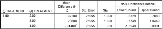
b. In general, when using two-way analysis of variance, if we find that there is an interaction effect, how does that affect the procedure?
188
views
 Verified step by step guidance
 06:28
06:28 06:50
06:50 06:33
06:33Interaction
b. In general, when using two-way analysis of variance, if we find that there is an interaction effect, how does that affect the procedure?
In Exercises 1–4, use the following listed measured amounts of chest compression (mm) from car crash tests (from Data Set 35 “Car Data” in Appendix B). Also shown are the SPSS results from analysis of variance. Assume that we plan to use a 0.05 significance level to test the claim that the different car sizes have the same mean amount of chest compression.
Anova
b. If the objective is to test the claim that the four car sizes have the same mean chest compression, why is the method referred to as analysis of variance?
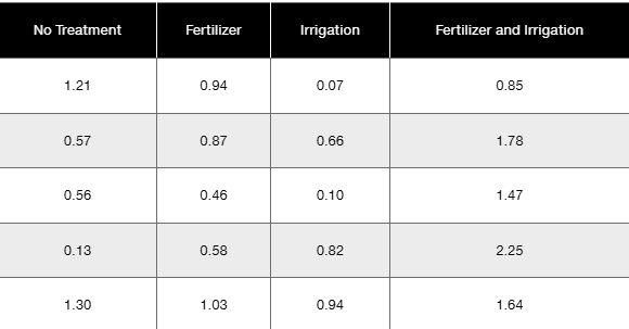
Transformations of Data Example 1 illustrated the use of two-way ANOVA to analyze the sample data in Table 12-3. How are the results affected in each of the following cases?
b. Each sample value is multiplied by the same nonzero constant.
In Exercises 1–5, refer to the following list of numbers of years that deceased U.S. presidents, popes, and British monarchs lived after their inauguration, election, or coronation, respectively. (As of this writing, the last president is George H. W. Bush, the last pope is John Paul II, and the last British monarch is George VI.) Assume that the data are samples from larger populations.
[Image]
Exploring the Data Include appropriate units in all answers.
d. Are there any obvious outliers?
c. Shown below is an interaction graph constructed from the data in Exercise 1. What does the graph suggest?
Transformations of Data Example 1 illustrated the use of two-way ANOVA to analyze the sample data in Table 12-3. How are the results affected in each of the following cases?
c. The format of the table is transposed so that the row and column factors are interchanged.