Chapter 3: Numerically Summarizing Data

3.1 Measures of Central Tendency

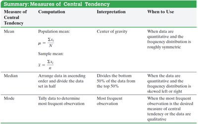
Measures of central tendency are statistical values that describe the center or typical value of a dataset. The three main measures are the mean, median, and mode.

Arithmetic Mean

• Definition: The arithmetic mean (or simply, the mean) is the sum of all values divided by the number of observations.

• Population Mean (\(\mu\)): where \(N\) is the population size.

• Sample Mean (\(\bar{x}\)): where \(n\) is the sample size.

• Interpretation: The mean is considered the "center of gravity" of the data.

• When to Use: When data are quantitative and the distribution is roughly symmetric.

Median

• Definition: The median is the value that lies in the middle of the data when arranged in ascending order.

• Computation Steps:

  1. Arrange data in ascending order.

  2. If the number of observations (n) is odd, the median is the middle value: position \(\frac{n+1}{2}\).

  3. If n is even, the median is the mean of the two middle values: positions \(\frac{n}{2}\) and \(\frac{n}{2} + 1\).

• Interpretation: Divides the bottom 50% of the data from the top 50%.

• When to Use: When the data are quantitative and the distribution is skewed left or right.

Mode

• Definition: The mode is the most frequent observation in the dataset.

• Computation: Tally the number of occurrences for each value; the value with the highest frequency is the mode.

• Interpretation: Most frequent observation.

• When to Use: When the most frequent observation is the desired measure or for qualitative data.

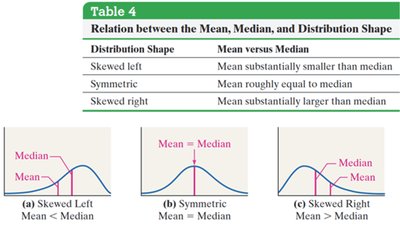
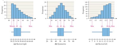
Relation Between Mean, Median, and Distribution Shape

• Skewed Left: Mean < Median

• Symmetric: Mean ≈ Median

• Skewed Right: Mean > Median

Resistant Statistics

• Definition: A statistic is resistant if it is not substantially affected by extreme values (outliers).

• Key Point: The median is resistant; the mean is not resistant.

• Example: Adding an extreme value to a dataset will change the mean more than the median.

3.2 Measures of Dispersion

Measures of dispersion describe the spread or variability of the data. Common measures include range, variance, and standard deviation.

Range

• Definition: The range is the difference between the largest and smallest data values.

• Formula: Range = Largest value – Smallest value

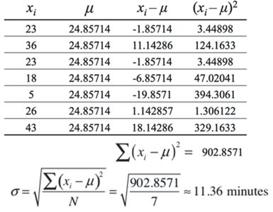
Standard Deviation

• Population Standard Deviation (\(\sigma\)):

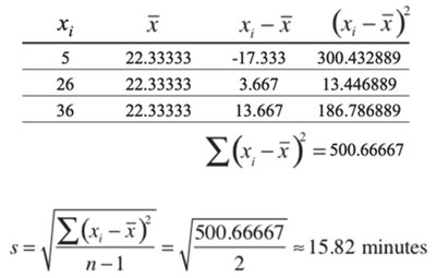
• Sample Standard Deviation (\(s\)):

• Interpretation: Measures the average distance of data values from the mean.

• Degrees of Freedom: For a sample, n – 1 is used in the denominator because the last value is determined by the others.

Variance

• Definition: The variance is the square of the standard deviation.

• Population Variance:

• Sample Variance:

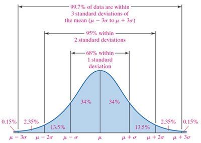
The Empirical Rule (for Bell-Shaped Distributions)

• Approximately 68% of data lie within 1 standard deviation of the mean.

• Approximately 95% within 2 standard deviations.

• Approximately 99.7% within 3 standard deviations.

• Formulas:

  • \(\mu \pm 1\sigma\): 68%

  • \(\mu \pm 2\sigma\): 95%

  • \(\mu \pm 3\sigma\): 99.7%

Chebyshev’s Inequality (for Any Distribution)

• For any data set, at least (as a proportion) of the data lie within k standard deviations of the mean, for any k > 1.

• Formula: At least of the data are within .

3.3 Measures from Grouped Data

When only grouped (frequency) data are available, we can approximate the mean and standard deviation.

Approximate Mean from Grouped Data

• Formula: , where is the class midpoint and is the class frequency.

Weighted Mean

• Formula: , where is the weight for observation .

Approximate Standard Deviation from Grouped Data

• Population:

• Sample:

3.4 Measures of Position and Outliers

Measures of position describe the relative standing of a value within a dataset.

z-Scores

• Population z-Score:

• Sample z-Score:

• Interpretation: Indicates how many standard deviations a value is from the mean.

Percentiles

• Definition: The kth percentile is the value below which k% of the data fall.

Quartiles

• Q1: 25th percentile (bottom 25%)

• Q2: 50th percentile (median)

• Q3: 75th percentile (bottom 75%)

• Computation: Arrange data, find median, then medians of lower and upper halves for Q1 and Q3.

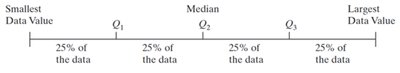
Interquartile Range (IQR)

• Definition: The range of the middle 50% of the data.

• Formula:

Checking for Outliers

• Calculate Q1, Q3, and IQR.

• Lower fence:

• Upper fence:

• Any value outside these fences is considered an outlier.

3.5 The Five-Number Summary and Boxplots

The five-number summary provides a concise description of a dataset and is the basis for constructing boxplots.

Five-Number Summary

• Minimum

• First Quartile (Q1)

• Median (Q2)

• Third Quartile (Q3)

• Maximum

Boxplots

• Visual representation of the five-number summary.

• Box extends from Q1 to Q3, with a line at the median.

• Whiskers extend to the smallest and largest values within the fences; outliers are plotted individually.

• Boxplots are useful for comparing distributions and identifying skewness and outliers.

Summary Table: Measures of Central Tendency

Summary Table: Relation Between Mean, Median, and Distribution Shape

Additional info: The above notes include all key definitions, formulas, and examples necessary for understanding and applying measures of central tendency, dispersion, position, and graphical summaries in statistics. The included images reinforce the concepts of distribution shape, calculation of standard deviation, the empirical rule, quartiles, and boxplots.