Probability in Our Daily Lives

Section 5.1: How Can Probability Quantify Randomness?

Random Phenomena

Random phenomena are events whose outcomes are uncertain in the short run, but exhibit predictable patterns in the long run. Probability is the mathematical tool used to quantify this long-run randomness.

• Definition: A phenomenon is random if individual outcomes are uncertain, but there is a regular distribution of outcomes in a large number of repetitions.

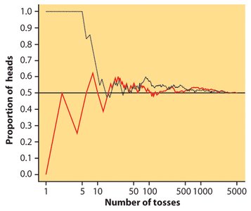
• Short-run vs. Long-run: In the short run, proportions are highly variable; in the long run, they stabilize.

• Probability: The probability of any outcome is the proportion of times the outcome would occur in a very long series of repetitions.

Law of Large Numbers

The Law of Large Numbers states that as the number of trials increases, the proportion of occurrences of any given outcome approaches a particular value.

• Example: Tossing a fair die many times, the proportion of sixes approaches .

Probability

Probability is the proportion of times a particular outcome occurs in a long run of observations.

• Example: Rolling a die, the probability of getting a 6 is .

Independent Trials

Trials are independent if the outcome of one trial does not affect the outcome of another. This is a key assumption in many probability calculations.

• Example: Coin flips are independent; the probability of heads remains regardless of previous outcomes.

• Sampling with replacement: Independence is maintained when each trial is performed with replacement.

Section 5.2: How Can We Find Probabilities?

Sample Space

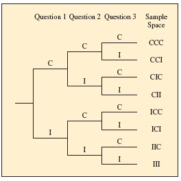
The sample space is the set of all possible outcomes for a random phenomenon.

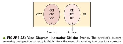
• Example: For three multiple-choice questions, the sample space includes all possible sequences of correct (C) and incorrect (I) answers.

Event

An event is a subset of the sample space, corresponding to a particular outcome or group of outcomes.

• Example: Event A: student answers all 3 questions correctly (CCC). Event B: student passes (at least 2 correct) = (CCI, CIC, ICC, CCC).

Probabilities for a Sample Space

Each outcome in a sample space has a probability between 0 and 1. The sum of all probabilities in the sample space equals 1.

• Discrete Sample Space: Contains a finite number of outcomes, such as dice rolls.

• Continuous Sample Space: Contains an infinite number of outcomes, such as weight gain measured in grams.

Calculating Probabilities

When all outcomes are equally likely, the probability of an event A is:

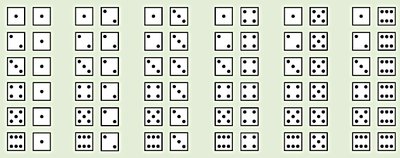
Example: Probability of Sum of Two Dice

There are 36 possible outcomes when rolling two dice. The probability that the sum is 5:

• Possible pairs: (1,4), (2,3), (3,2), (4,1)

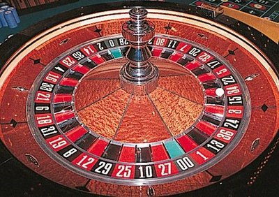
Applications: Gambling Industry

The gambling industry uses probability distributions to calculate odds and set rewards, ensuring profitability for the house.

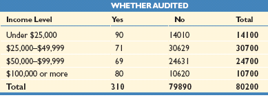
Example: Probability of Being Audited

Sample space for selecting a taxpayer includes combinations of income level and audit status. Probabilities can be calculated from observed frequencies.

Types of Probability: Relative Frequency vs. Subjective

• Relative Frequency: Probability is the long-run proportion of times an outcome occurs in repeated trials.

• Subjective Probability: When repeated trials are not feasible, probability is based on degree of belief, often used in Bayesian statistics.

Rules for Finding Probabilities About Pairs of Events

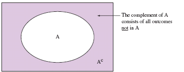
Complement of an Event

The complement of event A, denoted Ac, consists of all outcomes in the sample space not in A. The probabilities of A and Ac add to 1.

Disjoint Events

Two events are disjoint if they have no outcomes in common.

• For disjoint events,

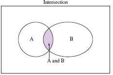
Intersection of Two Events

The intersection of events A and B consists of outcomes that are in both A and B.

• is the probability that both events occur.

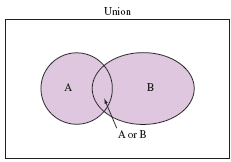
Union of Two Events

The union of events A and B consists of outcomes that are in A, B, or both.

• is the probability that at least one event occurs.

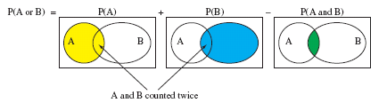
Addition Rule for Probability

For any two events A and B:

• If A and B are disjoint:

Example: Probability of Audit and High Income

• Event A: being audited

• Event B: income greater than $100,000

Multiplication Rule for Intersection of Independent Events

For independent events A and B:

Example: Probability of Correct Answers by Guessing

• Probability of guessing correctly: 0.2

• Probability of getting all three correct:

• Probability of at least two correct:

Events Often Are Not Independent

Independence should not be assumed without careful consideration. Real-world data often show dependence between events.

• Example: Pop quiz with two questions. Actual probabilities for outcomes:

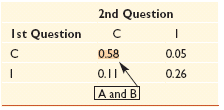
• Define A: first question correct; B: second question correct

• If independent: (but actual is 0.58)

Summary Table: Probability Concepts

Key Takeaways

• Probability quantifies randomness and is foundational to statistical inference.

• Understanding sample spaces, events, and probability rules is essential for analyzing random phenomena.

• Careful consideration of independence and real-world data is necessary for accurate probability calculations.