 Back
BackChapter 6: Modeling Random Events – The Normal and Binomial Models
Study Guide - Smart Notes
 Tailored notes based on your materials, expanded with key definitions, examples, and context.
Chapter 6: Modeling Random Events – The Normal and Binomial Models
Random Variables
Random variables are fundamental in statistics for modeling outcomes of random phenomena. A random variable, denoted as X, is a variable whose values are numerical outcomes of a random process.
Discrete Random Variable: Takes countable values, usually whole numbers. Examples:
X = number of heads in 3 coin tosses
Y = number of hits a website gets in a day
Z = number of customers arriving at a bank from 1-2 pm
Continuous Random Variable: Takes measurable values, including decimals. These cannot be listed or counted because they occur over a range. Examples:
X = time it takes for the next bus to come
Y = amount of rain in Portland during March
Z = weight of a cow
Identifying Discrete and Continuous Variables
It is important to distinguish between discrete and continuous variables in practice:
a) Number of cars owned by a household – Discrete
b) Time it takes a worker to commute to a job site – Continuous
c) Height of a building in downtown SF – Continuous
d) Number of pets owned by a student – Discrete
Discrete Probability Distributions
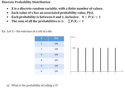
A discrete probability distribution describes the probabilities of outcomes for a discrete random variable.
X is a discrete random variable with a finite number of values.
Each value of X has an associated probability P(x).
Each probability is between 0 and 1:
The sum of all probabilities is 1:
Example: Let X = outcome of a roll of a die.
x | P(x) |
|---|---|
1 | 1/6 |
2 | 1/6 |
3 | 1/6 |
4 | 1/6 |
5 | 1/6 |
6 | 1/6 |
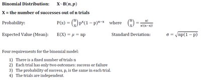
Binomial Distribution
The binomial distribution models the number of successes in a fixed number of independent trials, each with the same probability of success.
X ~ B(n, p): X is the number of successes out of n trials
Probability: , where
Expected Value (Mean):
Standard Deviation:
Requirements for the binomial model:
Fixed number of trials n
Each trial has two outcomes: success or failure
Probability of success p is the same in each trial
Trials are independent
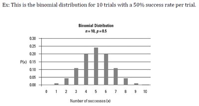
Example: Binomial Distribution for 10 Trials
For n = 10, p = 0.5, the binomial distribution shows the probability of each possible number of successes.
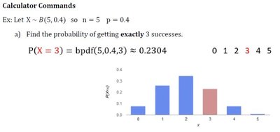
Calculator Commands for Binomial Probabilities
Statistical calculators can compute binomial probabilities using functions such as bpdf (binomial probability density function) and bcdf (binomial cumulative density function).
Probability of exactly k successes:
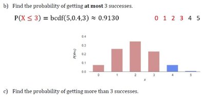
Probability of at most k successes:
Probability of more than k successes:
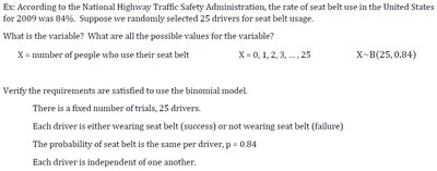
Application Example: Seat Belt Usage
Suppose the seat belt usage rate is 84% and we randomly select 25 drivers. The binomial model can be used to calculate expected values and probabilities.
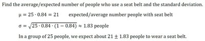
Expected number:
Standard deviation:
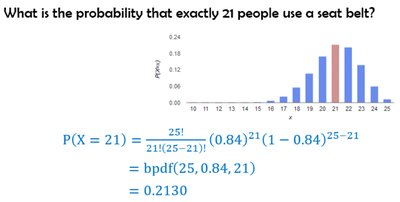
Probability that exactly 21 people use a seat belt:
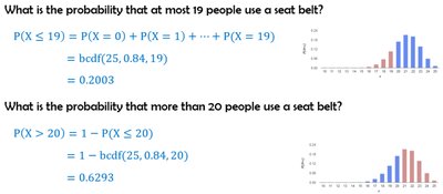
Probability that at most 19 people use a seat belt:
Probability that more than 20 people use a seat belt:
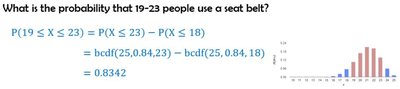
Probability that 19–23 people use a seat belt:
Other Binomial Examples
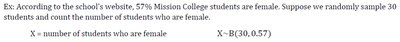
Sampling students for gender or calculating expected hits for a baseball player can also be modeled using the binomial distribution.
For 30 students, 57% female:
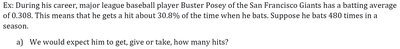
For a player with a batting average of 0.308 and 480 at-bats: Expected hits
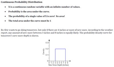
Continuous Probability Distributions
A continuous probability distribution describes probabilities for a continuous random variable. Probability is represented by the area under the curve, not by individual values.
X is a continuous random variable with an infinite number of values.
Probability is the area under the curve.
The probability of a single value is zero.
Total area under the curve must be 1.
Example: Probability density curve for new snow depth between 3 and 8 inches.
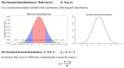
The Normal Distribution
The normal distribution is a continuous random variable with a symmetric, bell-shaped curve. It is defined by its mean () and standard deviation ().
Notation:
The standard normal distribution is
To convert X to Z, use the z-score formula:
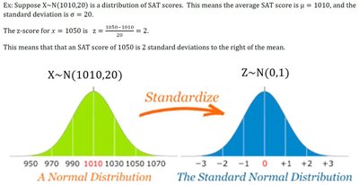
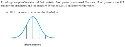
Normal Distribution Examples
Examples include SAT scores, blood pressure, and other measurements that follow a normal distribution.
For SAT scores: ,
For blood pressure: Mean = 125 mmHg, SD = 10 mmHg
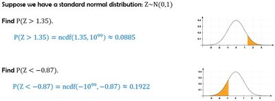
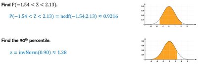
Calculating Probabilities with the Standard Normal Distribution
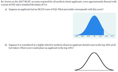
Probabilities can be found using the cumulative distribution function (ncdf) and inverse normal function (invNorm).
90th percentile:
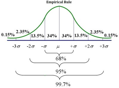
The Empirical Rule
The empirical rule describes the percentage of values within 1, 2, and 3 standard deviations of the mean in a normal distribution:
68% within 1 SD
95% within 2 SD
99.7% within 3 SD
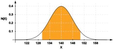
Normal Distribution Applications
Applications include defining random variables and distributions, calculating probabilities for ranges, and determining percentiles.
Weight of students:
Probability for a range: Area under the curve between two values
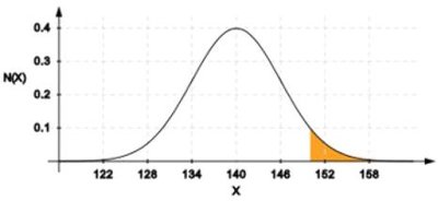
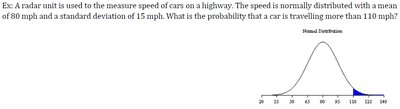
Probability for values above a threshold: Area to the right of a value

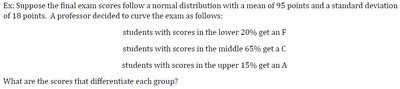
Curving Exam Scores Using Normal Distribution
Normal distributions can be used to curve exam scores by assigning grades based on percentiles.
Lower 20%: F
Middle 65%: C
Upper 15%: A
 Additional info: The notes cover all major aspects of Chapter 6, including random variables, discrete and continuous probability distributions, binomial and normal models, and practical applications with calculator commands and real-world examples.
