Chi-Square Tests & Goodness of Fit

Overview of the Chi-Square Test

The Chi-square test is a statistical method used to determine if there is a significant association between categorical variables. It is commonly applied to contingency tables to test hypotheses about relationships between variables such as survival rates and passenger class.

• Null Hypothesis (H0): No association exists between the variables.

• Alternative Hypothesis (Ha): An association exists between the variables.

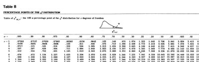
• Test Statistic: The Chi-square statistic is calculated as: where O is the observed frequency and E is the expected frequency.

• Critical Value: Compare the calculated statistic to the critical value from the Chi-square distribution table at the chosen significance level (e.g., 5%).

Titanic Example: Association Between Passenger Class and Survival

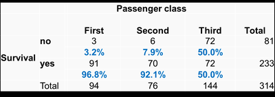
The Titanic dataset is used to test whether passenger class affected survival rates.

• Observed and expected frequencies are calculated for each class and survival outcome.

• Chi-square statistic is computed and compared to the critical value.

• Result: The null hypothesis is rejected, indicating a strong association between passenger class and survival.

Observed Frequencies Table

Expected Frequencies Table

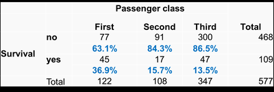
Effect of Gender on Survival

Survival rates are further analyzed by gender and passenger class.

• Female Passengers: Higher survival rates across all classes.

• Male Passengers: Lower survival rates, especially in third class.

Assumptions of the Chi-Square Test

For the Chi-square test to be valid:

• No more than 20% of the cells should have expected frequencies less than 5.

• If this condition is violated, categories may be combined to reduce the table size.

Example: Social and Economic Status for Married Couples

Grouped Table (for valid test)

Simpson’s Paradox

Definition and Example

Simpson’s Paradox occurs when a trend appears in several groups of data but disappears or reverses when the groups are combined. This paradox highlights the importance of considering confounding variables before drawing conclusions.

• Example: University of Berkeley admissions data initially suggested gender discrimination, but further analysis showed that females applied more to departments with lower admission rates.

• Another example: A study on heart disease and smoking showed higher survival rates for smokers, but confounding factors may explain this counter-intuitive result.

Berkeley Admissions Table

Assessing the Accuracy of Prediction Results

Confusion Matrix and Performance Metrics

In predictive modeling, accuracy is assessed using a confusion matrix, which compares predicted and actual outcomes.

• True Positive (TP): Correctly predicted positive cases

• True Negative (TN): Correctly predicted negative cases

• False Positive (FP): Incorrectly predicted positive cases

• False Negative (FN): Incorrectly predicted negative cases

Example: Fraud Detection

• Sensitivity (True Positive Rate):

• Specificity (True Negative Rate):

• Positive Predictive Value:

Example: Diagnostic Accuracy

• Sensitivity:

• Specificity:

• Positive Predictive Value:

Summary

• Validity of Chi-square Test: Requires sufficient sample size and expected frequencies.

• Simpson’s Paradox: Associations must be interpreted with caution, considering confounding variables.

• Prediction Accuracy: Evaluated using sensitivity, specificity, and positive predictive value from confusion matrices.