Confidence Intervals for a Population Mean

Overview

This section introduces the concept of confidence intervals for estimating a population mean, focusing on the Central Limit Theorem (CLT), sampling distributions, and the use of Z and t-distributions for interval estimation. Understanding these concepts is essential for making inferences about population parameters based on sample data.

Central Limit Theorem (CLT) and Sampling Distribution of the Mean

Central Limit Theorem

The Central Limit Theorem (CLT) states that, for a sufficiently large sample size (typically n > 30), the distribution of the sample mean (\( \overline{X} \)) will be approximately normal, regardless of the shape of the population distribution. The mean of this sampling distribution is the population mean (\( \mu \)), and its standard deviation is called the standard error:

• Standard Error of the Mean: \( \text{SE} = \frac{\sigma}{\sqrt{n}} \)

• Sampling Error: The difference between the sample mean and the population mean, \( \overline{x} - \mu \).

• Influences on Sampling Error:

  • Larger sample size decreases sampling error.

  • Higher dispersion (variance) increases sampling error.

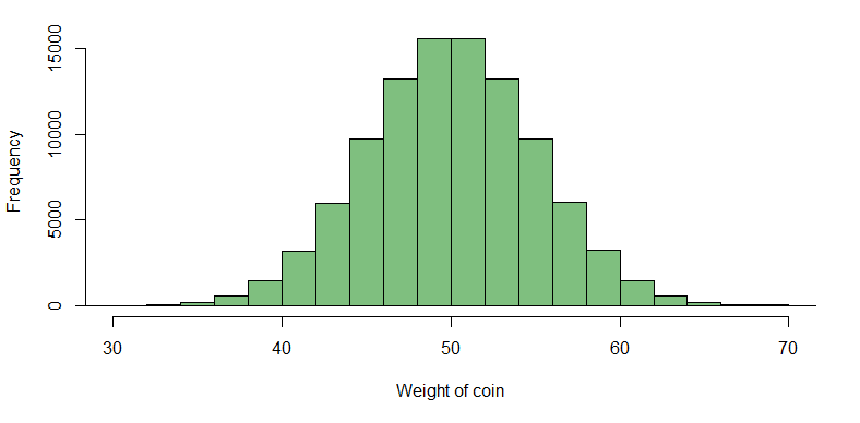
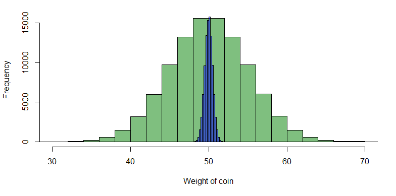
Sampling Distribution Example

Suppose the weight of genuine gold coins is normally distributed with mean 50g and standard deviation 5g. If we take repeated samples of 100 coins and calculate their means, the distribution of these means will also be normal, centered at 50g, but with a much smaller standard error.

Constructing Confidence Intervals for a Population Mean

General Form

A confidence interval provides a range of plausible values for an unknown population parameter. The general form is:

• Point Estimate ± (Critical Value) × (Standard Error)

For a population mean, the confidence interval depends on whether the population standard deviation (\( \sigma \)) is known and the sample size:

• Large sample (n > 30), \( \sigma \) known:

  • \( \overline{X} \pm z^* \frac{\sigma}{\sqrt{n}} \)

• Large sample (n > 30), \( \sigma \) unknown:

  • \( \overline{X} \pm z^* \frac{s}{\sqrt{n}} \)

• Small sample (n < 30), \( \sigma \) unknown:

  • \( \overline{X} \pm t^* \frac{s}{\sqrt{n}} \)

Where z* is the critical value from the standard normal distribution, and t* is from the Student t-distribution with n-1 degrees of freedom.

Interpreting Confidence Intervals

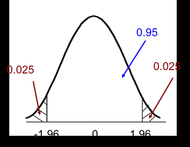
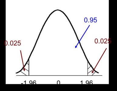
• Under repeated sampling, 95% of confidence intervals constructed in this way will contain the true population mean.

• We are 95% confident that the true population mean lies within the calculated interval.

• For other confidence levels, use the appropriate critical value (e.g., 1.64 for 90%, 2.58 for 99%).

Worked Examples

Example 1: Large Sample, Unknown Population Standard Deviation

Scenario: A water company wants to estimate the average cost of fitting water meters. From a sample of 50 houses, the mean cost is 115, standard deviation is 14.5.

• \( \overline{x} = 115 \)

• \( s = 14.5 \)

• \( n = 50 \)

95% Confidence Interval:

• \( 115 \pm 1.96 \times \frac{14.5}{\sqrt{50}} \)

• \( 115 \pm 4.02 \)

• Interval: (110.98, 119.02)

Interpretation: The average cost per meter for all Irish houses is estimated to be between 110.98 and 119.02, with 95% confidence.

Example 2: Testing a Company Claim

Scenario: Weight Reducers International claims an average weight loss of 4kg/month. A sample of 50 customers has a mean loss of 3.5kg, standard deviation 1.4kg.

• \( \overline{x} = 3.5 \)

• \( s = 1.4 \)

• \( n = 50 \)

95% Confidence Interval:

• \( 3.5 \pm 1.96 \times \frac{1.4}{\sqrt{50}} = 3.5 \pm 0.39 \)

• Interval: (3.11, 3.89)

Interpretation: The confidence interval does not include 4kg, so the data does not support the company's claim.

Confidence Intervals with Small Samples: The Student t-Distribution

When to Use the t-Distribution

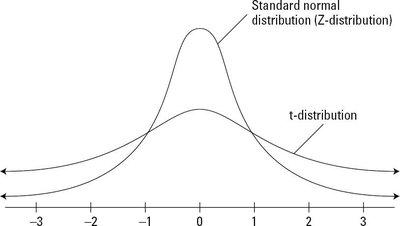
When the sample size is small (n < 30) and the population standard deviation is unknown, use the Student t-distribution. The t-distribution is wider than the normal distribution, reflecting greater uncertainty with small samples. As sample size increases, the t-distribution approaches the normal distribution.

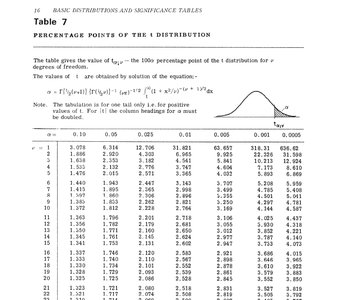
Finding the t-Value

• Degrees of freedom: \( v = n - 1 \)

• For a 95% confidence interval, use \( \alpha = 0.025 \) in each tail.

• Find the t-value in statistical tables for the appropriate degrees of freedom.

Example: Small Sample

Scenario: A sample of 25 cafes in Limerick has a mean cappuccino price of €3.85, standard deviation €0.53. Data is approximately normal.

• \( \overline{x} = 3.85 \)

• \( s = 0.53 \)

• \( n = 25 \)

• \( t_{24, 0.025} = 2.064 \)

95% Confidence Interval:

• \( 3.85 \pm 2.064 \times \frac{0.53}{\sqrt{25}} = 3.85 \pm 0.22 \)

• Interval: (3.63, 4.07)

Interpretation: The mean price of a take-away cappuccino in Limerick is estimated to be between €3.63 and €4.07 with 95% confidence.

Comparing Groups Using Confidence Intervals

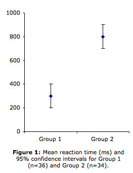
Identifying Differences

Confidence intervals can be used to compare means between groups. If the intervals do not overlap, it suggests a significant difference between the groups.

Summary Table: Confidence Intervals for a Mean

Key Terms: - Point Estimate: A single value estimate of a population parameter (e.g., sample mean). - Standard Error: The estimated standard deviation of a sample statistic. - Critical Value: The value from the Z or t-distribution corresponding to the desired confidence level. - Confidence Level: The probability that the interval contains the true parameter value (e.g., 95%).