Confidence Intervals for a Population Proportion

Introduction

Estimating the proportion of a population that possesses a certain characteristic is a fundamental task in statistics, especially when dealing with categorical data. Confidence intervals provide a range of plausible values for the true population proportion based on sample data, allowing for quantification of uncertainty in estimation.

Sampling Distribution of a Sample Proportion

Definition and Properties

• Sample Proportion (\( \hat{p} \)): The proportion of observations in a sample that fall into a specified category.

• Population Proportion (\( p \)): The true proportion of the population with the characteristic of interest.

• Sampling Distribution: If repeated random samples of size \( n \) are taken from a population with proportion \( p \), the distribution of the sample proportions \( \hat{p} \) is approximately normal for large \( n \), with mean \( p \) and standard deviation \( \sqrt{\frac{p(1-p)}{n}} \).

• This approximation is best when \( n \) is large and \( p \) is not close to 0 or 1.

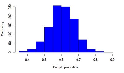
Example: If the true proportion of a population supporting a candidate is 0.62, and samples of size 40 are repeatedly taken, the sample proportions will be distributed approximately normally around 0.62.

Constructing a 95% Confidence Interval for a Population Proportion

Formula and Interpretation

• The general form for a 95% confidence interval for a population proportion is:

• Where:

  • \( \hat{p} \) = sample proportion

  • \( n \) = sample size

  • 1.96 is the z-value corresponding to a 95% confidence level

• The interval provides a range in which the true population proportion is likely to fall, with 95% confidence.

Example: In a consumer test, 56 out of 80 people reported improvement from a product. The sample proportion is \( \hat{p} = \frac{56}{80} = 0.70 \). The 95% confidence interval is:

Sample Size Calculation for a Desired Confidence Interval Width

Determining Required Sample Size

• To estimate a population proportion within a specified margin of error (E) at a given confidence level, the required sample size \( n \) can be calculated as:

• \( p^* \) is a prior estimate of the proportion (often 0.5 for maximum variability if unknown).

• For a 95% confidence interval, \( z = 1.96 \); for a 99% confidence interval, \( z = 2.58 \).

Example: To estimate a proportion to within 2% (E = 0.02) with 99% confidence and no prior estimate, use \( p^* = 0.5 \):

Worked Examples

Example 1: Confidence Interval Calculation

• Scenario: 120 out of 250 gift vouchers expired unused.

• \( \hat{p} = \frac{120}{250} = 0.48 \)

• 95% CI:

• Interpretation: We are 95% confident that the true proportion of expired vouchers is within the calculated interval.

Example 2: Hypothesis Testing Using Confidence Interval

• Question: Is there evidence that at least 40% of vouchers expire unused?

• If the lower bound of the confidence interval is above 0.40, there is evidence to support the claim.

Example 3: Changing Confidence Levels

• For a 99% confidence interval, replace 1.96 with 2.58 in the formula:

Summary Table: Sample Size and Error

The following table shows how sample size affects the margin of error for a 95% confidence interval when \( p = 0.5 \):

Key Points

• Confidence intervals for proportions are based on the normal approximation to the sampling distribution of \( \hat{p} \).

• The width of the interval depends on the sample size and the estimated proportion.

• For different confidence levels, use the appropriate z-value (e.g., 1.96 for 95%, 2.58 for 99%).

• Sample size calculations ensure the desired precision in estimation.