Continuous Probability Distributions

Introduction to Continuous Probability Distributions

Continuous probability distributions describe the probabilities of the possible values of a continuous random variable. Unlike discrete distributions, continuous distributions can take on infinitely many values within a given interval. The probability of the random variable falling within a particular interval is represented by the area under the curve of its probability density function (pdf).

• Probability Density Function (pdf): A function that describes the likelihood of a random variable to take on a particular value. For a function to be a valid pdf, it must satisfy:

  • The total area under the curve must equal 1.

  • The function must be non-negative for all values of the random variable.

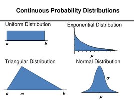
The Uniform Distribution

Definition and Properties

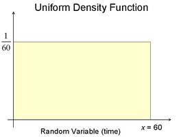
The uniform distribution is a type of continuous probability distribution where all intervals of the same length within the distribution's range are equally probable. It is defined by two parameters, a and b, which are the minimum and maximum values, respectively.

• Probability Density Function: For a uniform distribution on the interval [a, b], the pdf is given by:

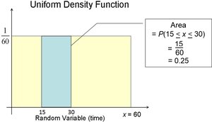
• Area Interpretation: The probability that the random variable falls within a certain interval is the area under the pdf over that interval.

Example: Package Delivery Time

Suppose a package is delivered between 10 am and 11 am, and the delivery time is equally likely at any minute in this interval. Let X be the number of minutes after 10 am. Then X is uniformly distributed on [0, 60].

• Probability Calculation: The probability that the package arrives between 15 and 30 minutes after 10 am is:

The Normal Distribution

Definition and Properties

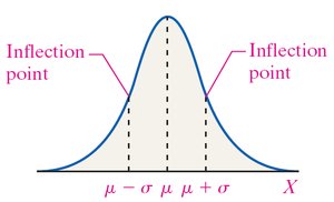
The normal distribution is a continuous probability distribution that is symmetric about its mean, μ, and characterized by its bell-shaped curve. It is one of the most important distributions in statistics due to the Central Limit Theorem and its frequent appearance in natural and social phenomena.

• Probability Density Function:

• Key Properties:

  • Symmetric about the mean μ

  • Mean = Median = Mode

  • Inflection points at μ - σ and μ + σ

  • Total area under the curve is 1

  • As x → ±∞, the curve approaches but never touches the x-axis

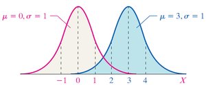
Effect of Mean and Standard Deviation

Changing the mean (μ) shifts the normal curve left or right, while changing the standard deviation (σ) affects the spread (width) of the curve but not its location.

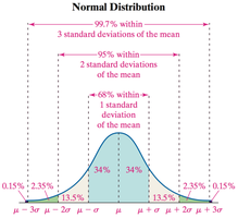
The Empirical Rule (68-95-99.7 Rule)

The Empirical Rule describes the proportion of data within certain standard deviations from the mean in a normal distribution:

• Approximately 68% of the data falls within 1 standard deviation (μ ± σ)

• Approximately 95% within 2 standard deviations (μ ± 2σ)

• Approximately 99.7% within 3 standard deviations (μ ± 3σ)

Applications of the Normal Distribution

The area under the normal curve for a given interval represents either the proportion of the population with a certain characteristic or the probability that a randomly selected individual has that characteristic.

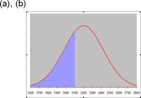
• Example: If giraffe weights are normally distributed with μ = 2200 lbs and σ = 200 lbs, and the area to the left of x = 2100 lbs is 0.3085, then:

  • 30.85% of giraffes weigh less than 2100 lbs

  • The probability that a randomly selected giraffe weighs less than 2100 lbs is 0.3085

The Standard Normal Distribution and Z-Scores

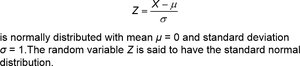
Standardization and Z-Scores

To compare values from different normal distributions, we standardize them using the z-score. The standard normal distribution has a mean of 0 and a standard deviation of 1. The z-score for a value x is:

Using the Standard Normal Table

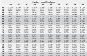
The Standard Normal Table (z-table) provides the area (probability) to the left of a given z-score under the standard normal curve. This allows us to find probabilities and percentiles for normally distributed variables after standardization.

• Example: Find the probability that a randomly chosen person has an IQ less than 120, given μ = 100 and σ = 15.

  • Calculate z:

  • Look up z = 1.33 in the z-table to find the area to the left (probability).

Finding Probabilities and Percentiles

• To find the probability that a value is greater than a certain value, subtract the area to the left from 1.

• To find the value corresponding to a given percentile, find the z-score for that percentile and solve for x using .

Assessing Normality

Normal Probability Plots

To determine if a data set is approximately normal, especially for small samples, we use a normal probability plot. This plot compares observed data values to expected z-scores. If the plot is approximately linear, the data are likely from a normal distribution.

• If the correlation coefficient between observed values and expected z-scores exceeds a critical value, normality is supported.

Summary Table: Key Properties of the Normal Distribution