Chapter 6: Discrete Probability Distributions

6.1 Discrete Random Variables

Discrete random variables are foundational in probability and statistics, representing outcomes that can be counted. This section distinguishes between discrete and continuous random variables, introduces probability distributions, and explains how to compute and interpret their mean and standard deviation.

Distinguishing Between Discrete and Continuous Random Variables

• Random Variable: A numerical measure of the outcome of a probability experiment, typically denoted by a capital letter (e.g., X).

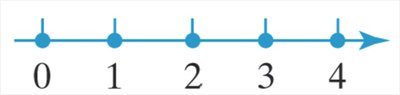
• Discrete Random Variable: Has a finite or countable number of values. These values can be plotted on a number line with gaps between points.

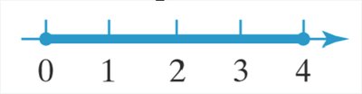
• Continuous Random Variable: Has infinitely many possible values, which can be plotted on a continuous line without gaps.

Example: Consider a bag of M&M’s:

• Mass of each M&M: Continuous (can take any value within a range)

• Number of pieces of candy: Discrete (countable whole numbers)

• Diameter of each piece: Continuous

• Number of distinct colors: Discrete

Identifying Discrete Probability Distributions

A discrete probability distribution lists each possible value of a discrete random variable and its probability. It can be represented as a table, graph, or formula.

• Rules for Discrete Probability Distributions:

  • All probabilities must sum to 1:

  • Each probability must be between 0 and 1:

Example: In the game Chuck-a-Luck, the random variable X represents the profit from a $1 bet. The probability distribution is:

Graphing Discrete Probability Distributions

Discrete probability distributions can be visualized using bar graphs, where the x-axis represents possible values and the y-axis represents probabilities.

Computing and Interpreting the Mean of a Discrete Random Variable

• Mean (Expected Value) Formula:

• The mean represents the long-run average outcome if the experiment is repeated many times.

Example: For the Chuck-a-Luck game, the mean profit is calculated using the table above.

Interpreting the Mean as an Expected Value

• The mean of a discrete random variable is also called the expected value, denoted .

• It predicts the average outcome over many repetitions of the experiment.

Example: If a property is resold at various prices with given probabilities, the expected profit can be calculated using the mean formula.

Computing the Standard Deviation of a Discrete Random Variable

• Standard Deviation Formula:

• Measures the spread of the distribution around the mean.

Example: For the Chuck-a-Luck game, use the table to compute the standard deviation.

6.2 The Binomial Probability Distribution

Determining Binomial Experiments

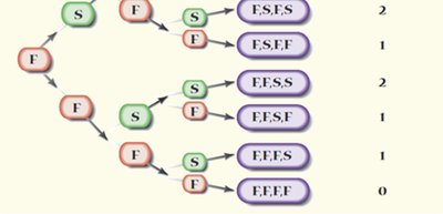
A binomial experiment is a specific type of probability experiment with the following criteria:

• Performed a fixed number of times (n trials)

• Trials are independent

• Each trial has two outcomes: success or failure

• Probability of success (p) is constant for each trial

Notation:

• n: number of trials

• p: probability of success

• X: number of successes in n trials

Computing Probabilities of Binomial Experiments

The probability of obtaining exactly x successes in n independent trials is given by the binomial probability formula:

where is the binomial coefficient.

Example: If 58% of Americans believe divorce is acceptable, in a sample of 30, the probability that exactly 20 do is found using the formula above.

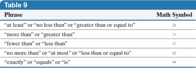
Interpreting Probability Phrases

Mean and Standard Deviation of a Binomial Random Variable

• Mean (Expected Value):

• Standard Deviation:

Example: In a sample of 500, if 58% believe divorce is acceptable, the mean and standard deviation are calculated using the formulas above.

Graphing Binomial Probability Distributions

As the number of trials n increases (with fixed p), the binomial distribution becomes more bell-shaped. If , the distribution is approximately normal.

Using the Mean, Standard Deviation, and Empirical Rule

To determine if an observed result is unusual, compare it to the mean and standard deviation. Results far from the mean (more than 2 standard deviations) are considered unusual.