Estimating Parameters and Determining Sample Sizes

Study Guide - Smart Notes

Tailored notes based on your materials, expanded with key definitions, examples, and context.

Estimating Parameters and Determining Sample Sizes

Estimating a Population Proportion

Estimating a population proportion involves using sample data to infer the value of a population parameter. The sample proportion is the best point estimate of the population proportion, and confidence intervals are constructed to provide a range of plausible values for the true population proportion.

Point Estimate: A single value used to approximate a population parameter. For proportions, the sample proportion \( \hat{p} \) is the best point estimate of the population proportion \( p \).
Formula: \( \hat{p} = \frac{x}{n} \), where \( x \) is the number of successes and \( n \) is the sample size.
Example: If 43% of 1487 surveyed adults have a Facebook page, the point estimate \( \hat{p} = 0.43 \).

Confidence Intervals for a Population Proportion

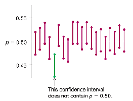
A confidence interval provides a range of values that is likely to contain the population proportion with a specified level of confidence. Common confidence levels are 90%, 95%, and 99%.

Confidence Level: The probability (1 − α) that the confidence interval contains the population parameter if the estimation process is repeated many times.
Interpretation: "We are 95% confident that the interval from 0.405 to 0.455 contains the true value of the population proportion \( p \)."
Process Success Rate: Over many samples, 95% of constructed confidence intervals will contain the true population proportion if the confidence level is 95%.

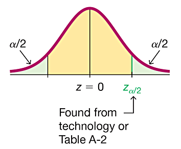
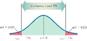
Confidence intervals from 20 samples, one not containing p=0.50

Critical Values and the Standard Normal Distribution

Critical values are z-scores that separate unlikely sample statistics from likely ones. The value \( z_{\alpha/2} \) is used to construct confidence intervals for proportions.

Critical Value: The z-score corresponding to the desired confidence level, found using statistical tables or technology.

Standard normal curve showing critical values z_alpha/2 Standard normal curve with confidence level and alpha regions

Common Critical Values

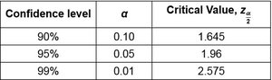
The table below lists common confidence levels and their corresponding critical values:

Confidence level	α	Critical Value, \( z_{\alpha/2} \)
90%	0.10	1.645
95%	0.05	1.96
99%	0.01	2.575

Table of common critical values for confidence intervals

Margin of Error for Proportions

The margin of error (E) quantifies the maximum likely difference between the sample proportion and the true population proportion at a given confidence level.

Formula:

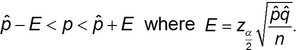
Formula for confidence interval and margin of error for proportions

Where \( \hat{q} = 1 - \hat{p} \), \( n \) is the sample size, and \( z_{\alpha/2} \) is the critical value.

Conditions for Constructing a Confidence Interval for Proportions

The sample must be a simple random sample.
The binomial distribution conditions are satisfied (fixed number of independent trials, two outcomes, constant probability).
There are at least 5 successes and 5 failures in the sample.

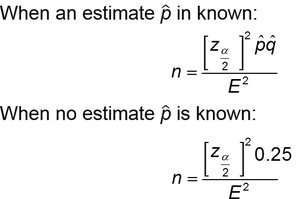
Determining Sample Size for Estimating a Population Proportion

To estimate a population proportion within a specified margin of error, the required sample size can be calculated using the following formulas:

When an estimate \( \hat{p} \) is known:

When no estimate \( \hat{p} \) is known:

Sample size formulas for estimating a population proportion

Estimating a Population Mean

Estimating a Population Mean (σ Not Known)

When the population standard deviation (σ) is unknown, the Student t distribution is used to construct confidence intervals for the population mean (μ). The t distribution accounts for the extra variability in small samples.

Degrees of Freedom (df): \( df = n - 1 \), where \( n \) is the sample size.
Margin of Error (E):

Where \( s \) is the sample standard deviation and \( t_{\alpha/2} \) is the critical t value.

Confidence Interval:

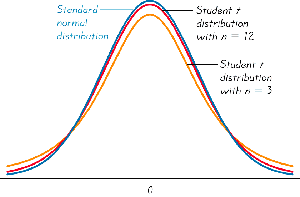
Properties of the Student t Distribution:
- Different for different sample sizes (n).
- Symmetric and bell-shaped, but wider than the normal distribution for small n.
- Mean of t = 0; standard deviation > 1 and varies with n.
- As n increases, the t distribution approaches the normal distribution.

Comparison of Student t distributions and standard normal distribution

Estimating a Population Mean (σ Known)

If the population standard deviation (σ) is known and the population is normally distributed or the sample size is large (n > 30), the normal (z) distribution is used.

Margin of Error (E):

Confidence Interval:

Choosing the Appropriate Distribution

Use the normal (z) distribution: σ known and population is normal or n > 30.
Use the t distribution: σ not known and population is normal or n > 30.
Use nonparametric methods or bootstrapping: Population is not normal and n ≤ 30.