Estimating Parameters and Determining Sample Sizes

Introduction

This chapter covers statistical methods for estimating population parameters, specifically proportions and means, using sample data. It also explains how to determine the sample size required for reliable estimation. The focus is on constructing and interpreting confidence intervals, understanding margin of error, and selecting appropriate distributions for inference.

Estimating a Population Proportion

Point Estimate

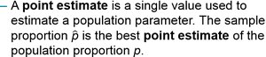
A point estimate is a single value used to estimate a population parameter. The sample proportion \( \hat{p} \) is the best point estimate of the population proportion \( p \).

• Unbiased Estimator: \( \hat{p} \) is unbiased and most consistent for estimating \( p \).

• Example: If 43% of 1487 adults in a poll have Facebook pages, the best point estimate of \( p \) is 0.43.

Confidence Interval

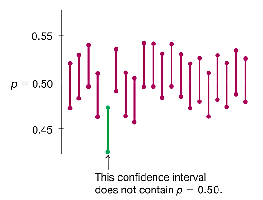
A confidence interval (CI) is a range of values used to estimate the true value of a population parameter. The confidence level (e.g., 95%) is the probability that the interval contains the parameter, assuming repeated sampling.

• Correct Interpretation: "We are 95% confident that the interval contains the true value of \( p \)."

• Process Success Rate: Over many samples, 95% of constructed intervals will contain the true \( p \).

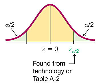
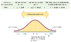
Critical Values

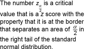
A critical value is a number separating significant sample statistics from those that are not. For confidence intervals, the critical value \( z_{\alpha/2} \) is a z-score at the border of an area \( \alpha/2 \) in the right tail of the standard normal distribution.

• For a 95% confidence level, \( \alpha = 0.05 \), so \( \alpha/2 = 0.025 \).

• \( z_{\alpha/2} = 1.96 \) for 95% confidence.

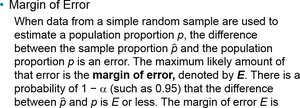
Margin of Error

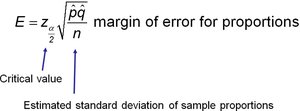
The margin of error (E) is the maximum likely difference between the sample proportion \( \hat{p} \) and the population proportion \( p \). It is calculated as:

• Formula:

• \( \hat{q} = 1 - \hat{p} \)

Confidence Interval for Population Proportion

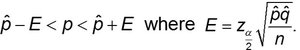
To estimate \( p \), construct the confidence interval:

• Formula:

• Requirements: Simple random sample, binomial conditions, at least 5 successes and 5 failures.

• Round interval limits to three significant digits.

Procedure for Constructing a Confidence Interval for p

1. Verify requirements (random sample, binomial conditions, minimum successes/failures).

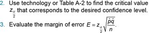
2. Find critical value \( z_{\alpha/2} \) for desired confidence level.

3. Calculate margin of error .

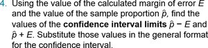
4. Compute interval limits: and .

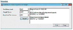
Example: Constructing a Confidence Interval

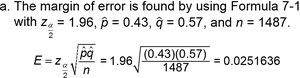
Given: 43% of 1487 adults have Facebook pages. Find the margin of error and 95% confidence interval.

• Margin of error:

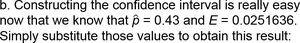
• Confidence interval: →

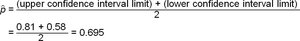
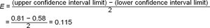
Finding Point Estimate and Margin of Error from a Confidence Interval

• Point estimate:

• Margin of error:

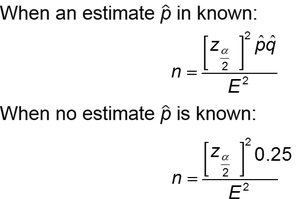
Determining Sample Size for Estimating a Population Proportion

To achieve a desired margin of error E at a given confidence level, use:

• With estimate \( \hat{p} \):

• Without estimate:

• Round up to next whole number.

Example: Sample Size Calculation

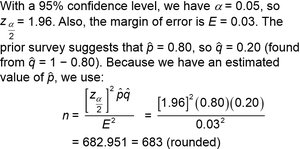
• With prior estimate \( \hat{p} = 0.80 \), \( \hat{q} = 0.20 \), \( z_{\alpha/2} = 1.96 \), \( E = 0.03 \):

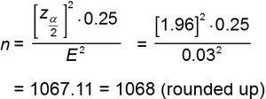
• Without prior estimate:

Estimating a Population Mean

Point Estimate and Confidence Interval for Mean

The main goal is to use a sample mean \( \bar{x} \) to infer the population mean \( \mu \). Confidence intervals are constructed differently depending on whether the population standard deviation \( \sigma \) is known or unknown.

Confidence Interval for Mean with Known σ

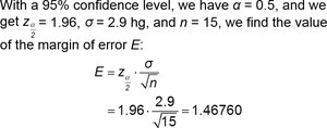
• Margin of error:

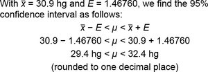
• Confidence interval:

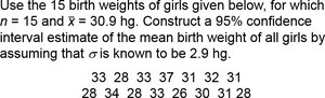
• Example: For \( \bar{x} = 30.9 \), \( \sigma = 2.9 \), \( n = 15 \), \( z_{\alpha/2} = 1.96 \):

• Interval: (rounded to one decimal place)

Confidence Interval for Mean with Unknown σ

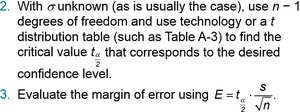
• Use Student t distribution with degrees of freedom \( df = n - 1 \).

• Margin of error:

• Confidence interval:

• Round limits to one more decimal place than original data.

Student t Distribution

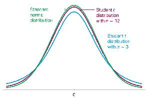
The Student t distribution is used when \( \sigma \) is unknown. It is similar to the normal distribution but has greater variability for small samples.

• Mean of t distribution is 0.

• Standard deviation varies with sample size and is greater than 1.

• As sample size increases, t distribution approaches normal distribution.

Procedure for Constructing a Confidence Interval for µ

1. Verify requirements: random sample, normal population or n > 30.

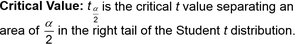
2. With unknown \( \sigma \), use t distribution and find critical value \( t_{\alpha/2} \).

3. Calculate margin of error .

4. Compute interval limits: and .

Finding Sample Size for Estimating a Population Mean

• Required sample size:

• If \( \sigma \) is unknown, estimate using range rule:

• Round up to next whole number.

Example: IQ Scores of Statistics Students

• Assume \( \sigma = 15 \), \( z_{\alpha/2} = 1.96 \), \( E = 3 \):

• Interpretation: At least 97 students are needed for 95% confidence that the sample mean is within 3 points of the population mean.

Choosing an Appropriate Distribution

Student t vs. Normal (z) Distribution

• Use z distribution when \( \sigma \) is known and sample size is large.

• Use t distribution when \( \sigma \) is unknown or sample size is small.

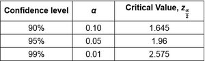
Summary Table: Common Critical Values

Key Terms and Notation

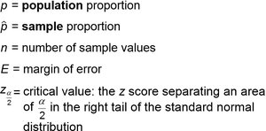
• p: Population proportion

• \( \hat{p} \): Sample proportion

• n: Number of sample values

• E: Margin of error

• zα/2: Critical value for z distribution

• tα/2: Critical value for t distribution

• \( \bar{x} \): Sample mean

• σ: Population standard deviation

• s: Sample standard deviation