Estimating Parameters and Determining Sample Sizes

Introduction to Estimation

In statistics, we often seek to infer characteristics of a population using data from a sample. The unknown numerical summary of a population is called a parameter, while any numerical measure computed from a sample is called a statistic. Since it is usually impractical to collect data from an entire population, we use sample statistics to estimate population parameters.

• Estimate: The best guess for the value of an unknown parameter, calculated using an estimator.

• Point Estimator: Provides a single value as an estimate of a parameter (e.g., sample mean \( \bar{x} \) for population mean \( \mu \)).

• Interval Estimator: Provides a range of values (interval) within which the parameter is expected to lie (e.g., confidence interval).

Confidence Intervals and Confidence Level

A confidence interval (CI) is a range of values, derived from sample statistics, that is likely to contain the value of an unknown population parameter. The confidence level is the probability that the interval estimate contains the true parameter value, commonly expressed as (1 − \( \alpha \)). Typical confidence levels are 90%, 95%, and 99%.

• Precision: Refers to the width of the confidence interval.

• Reliability: Refers to the confidence level.

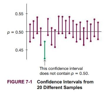
For example, a 95% confidence interval means that if we were to take 20 different samples and compute a confidence interval from each, we would expect about 19 of those intervals to contain the true parameter value.

Estimating a Population Proportion

Point and Interval Estimates for Proportion

The sample proportion (\( \hat{p} \)) is the best point estimate for the population proportion (\( p \)). The confidence interval for a population proportion is calculated as follows:

• \( \hat{p} = \frac{x}{n} \), where x is the number of successes and n is the sample size.

• Margin of Error: \( E = z_{\alpha/2} \sqrt{ \frac{ \hat{p}(1-\hat{p}) }{ n } } \)

• Confidence Interval: \( \hat{p} - E < p < \hat{p} + E \) or \( (\hat{p} - E, \hat{p} + E) \)

Requirements for using this method:

• Simple random sample

• Binomial distribution conditions are met

• At least 5 successes and 5 failures (\( np \geq 5 \) and \( nq \geq 5 \))

Example: Constructing a Confidence Interval for a Proportion

• Suppose in a survey of 500 drivers, 230 reported swerving while talking on a cell phone.

• \( \hat{p} = \frac{230}{500} = 0.46 \)

• For a 90% confidence level, \( z_{\alpha/2} = 1.645 \)

• \( E = 1.645 \times \sqrt{ \frac{0.46 \times 0.54}{500} } = 0.037 \)

• 90% CI: (0.423, 0.497)

Interpretation: We are 90% confident that the true proportion of drivers who have had to swerve while talking on a cell phone is between 42.3% and 49.7%.

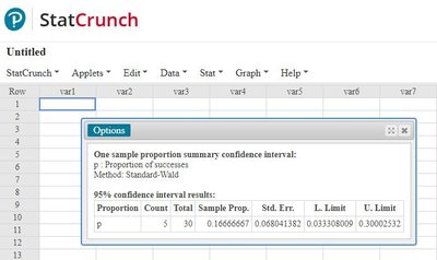
Using StatCrunch for Confidence Intervals

StatCrunch can be used to compute confidence intervals for proportions efficiently. The output provides the sample proportion, standard error, and the lower and upper limits of the confidence interval.

Effect of Confidence Level on Interval Width

Increasing the confidence level (e.g., from 95% to 99%) results in a wider confidence interval, reflecting greater uncertainty but higher reliability.

Finding Point Estimate and Margin of Error from a Confidence Interval

• Point Estimate: \( \hat{p} = \frac{\text{Upper Limit} + \text{Lower Limit}}{2} \)

• Margin of Error: \( E = \frac{\text{Upper Limit} - \text{Lower Limit}}{2} \)

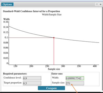
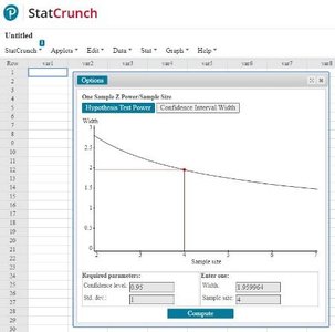
Determining Sample Size for Estimating a Proportion

To estimate the required sample size for a desired margin of error and confidence level:

• If \( \hat{p} \) is known:

• If \( \hat{p} \) is unknown, use 0.5 for maximum variability:

• Always round up to the next whole number.

Estimating a Population Mean

Estimating the Mean When Population Standard Deviation is Unknown

When the population standard deviation (\( \sigma \)) is unknown, we use the sample standard deviation (\( s \)) and the Student's t-distribution to construct confidence intervals for the population mean (\( \mu \)).

• Point Estimate: \( \bar{x} \) (sample mean)

• Standardized Variable: This follows a t-distribution with \( n-1 \) degrees of freedom if the population is normal or \( n > 30 \).

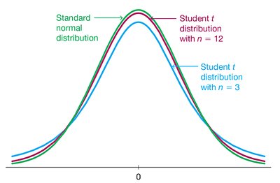
Student's t-Distribution

• Symmetric and bell-shaped, like the standard normal distribution, but with heavier tails.

• As sample size increases, the t-distribution approaches the standard normal distribution.

Confidence Interval for the Mean (\( \sigma \) Unknown)

• Requirements:

  • Simple random sample

  • Population is normal or sample size \( n > 30 \)

• Formula:

• Margin of Error:

Example: Confidence Interval for a Mean

• Sample size: 36, Sample mean: 50, Sample standard deviation: 20

• 90% confidence level, \( t_{\alpha/2} = 1.69 \)

• \( E = 1.69 \times \frac{20}{\sqrt{36}} = 5.633 \)

• 90% CI: (44.367, 55.633)

Interpretation: We are 90% confident that the true mean approval process time is between 44.4 and 55.6 days.

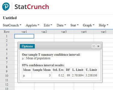
Using StatCrunch for Confidence Intervals for Means

StatCrunch provides tools for calculating confidence intervals for means using the t-distribution. The output includes the sample mean, standard error, degrees of freedom, and the confidence interval limits.

Determining Sample Size for Estimating a Mean

• Formula:

• If \( n \) is not a whole number, round up to the next integer.

Summary Table: Key Formulas

Additional info: StatCrunch is a statistical software tool that simplifies the calculation of confidence intervals and sample sizes for both proportions and means. The screenshots provided illustrate its use for these calculations.