7.1 Estimating Population Proportions and Determining Sample Sizes

Study Guide - Smart Notes

Tailored notes based on your materials, expanded with key definitions, examples, and context.

Chapter 7: Estimating Parameters and Determining Sample Sizes

Introduction to Inferential Statistics

Inferential statistics involves using sample data to make inferences or draw conclusions about population parameters. This chapter focuses on estimating population proportions and means, and determining the appropriate sample size for such estimations.

Estimation: Using sample data to estimate population parameters (such as proportions and means).
Hypothesis Testing: Using sample data to test claims about population parameters (covered in later chapters).

Estimating a Population Proportion

Point Estimate

A point estimate is a single value used to approximate a population parameter. For population proportions, the sample proportion $ \hat{p} $ is the best point estimate of the population proportion $ p $.

Unbiased Estimator: A statistic whose sampling distribution has a mean equal to the population parameter it estimates. $ \hat{p} $ is unbiased for $ p $.
Example: In a survey of 950 students, 53% take online courses. The best point estimate of the proportion of all students who take online courses is 0.53.

Confidence Interval (CI)

A confidence interval is a range of values used to estimate the true value of a population parameter. It consists of two main elements:

Confidence Level: The probability (e.g., 95%) that the CI contains the population parameter.
Margin of Error (E): The maximum likely difference between the sample statistic and the population parameter.

Relationship Between Confidence Level and $ \alpha $

Confidence Level	$ \alpha $
90%	0.10
95%	0.05
99%	0.01

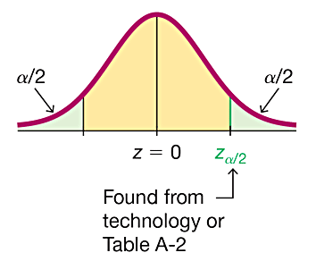
Critical Values

The critical value is the z-score that separates the central area from the tails in the standard normal distribution, corresponding to the desired confidence level.

$Standard normal distribution with critical values z_{\alpha/2}$ Finding the critical value for a 95% confidence level

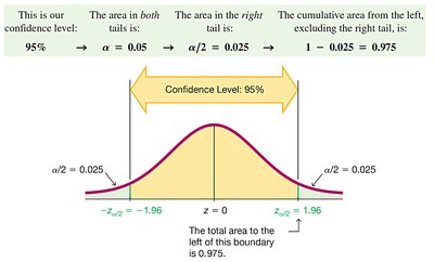
Confidence Level	$ \alpha $	Critical Value $ z_{\alpha/2} $
90%	0.10	1.645
95%	0.05	1.96
99%	0.01	2.575

$Critical value for 95% confidence level is z_{\alpha/2} = 1.96$

Margin of Error for Proportions

The margin of error (E) for estimating a population proportion is calculated as:

Where $ \hat{q} = 1 - \hat{p} $, $ n $ is the sample size, and $ z_{\alpha/2} $ is the critical value.
This is known as the Wald confidence interval.

Interpreting Confidence Intervals

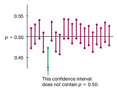
Correct interpretation: "We are 95% confident that the interval from 0.405 to 0.455 contains the true population proportion $ p $." This means that if we repeated the sampling process many times, 95% of the constructed intervals would contain $ p $.

Incorrect: "There is a 95% chance that $ p $ is between 0.405 and 0.455." (The parameter is fixed; the interval is random.)
Incorrect: "95% of sample proportions will fall between 0.405 and 0.455."

Confidence intervals from 20 samples, showing coverage probability

Constructing a Confidence Interval for $ p $

To construct a confidence interval for a population proportion:

Verify requirements: simple random sample, binomial conditions, at least 5 successes and 5 failures.
Find the critical value $ z_{\alpha/2} $.
Calculate the margin of error $ E $.
Compute the interval: $ \hat{p} - E < p < \hat{p} + E $.
Round limits to three significant digits.

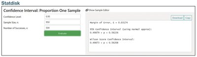
Example: Online Courses

Sample size: $ n = 950 $
Sample proportion: $ \hat{p} = 0.53 $
Critical value for 95% CI: $ z_{\alpha/2} = 1.96 $
Margin of error:
Confidence interval: or

Statdisk output for confidence interval calculation

Analyzing Polls

Sample should be a simple random sample.
Confidence level and sample size should be reported.
Population size is usually not a factor in reliability; sample size and method are more important.

Finding Point Estimate and Margin of Error from a Confidence Interval

Point estimate:
Margin of error:

Determining Sample Size for Estimating a Proportion

To estimate a population proportion with a specified margin of error and confidence level, the required sample size $ n $ is:

If an estimate of $ \hat{p} $ is known:
If no estimate is known (use maximum variability, $ \hat{p} = 0.5 $):
Always round up to the next whole number.

Example: Online Purchases

Prior estimate: $ \hat{p} = 0.79 $, $ \hat{q} = 0.21 $, $ E = 0.03 $, $ z_{\alpha/2} = 1.96 $
No prior estimate:

Alternative Confidence Interval Methods

Coverage Probability

The coverage probability of a confidence interval is the actual proportion of intervals that contain the true parameter. The Wald CI often has lower coverage probability than the nominal confidence level, especially for small samples or proportions near 0 or 1.

Better Performing Confidence Intervals

Plus Four Method: Add 2 to the number of successes and 2 to the number of failures, then use the Wald formula. This improves coverage probability.
Wilson Score Interval: More complex, but coverage probability is closer to the nominal level. Formula:
Clopper-Pearson Method: An exact method based on the binomial distribution; tends to be conservative (actual coverage probability is at least the nominal level).

Summary Table: Confidence Interval Methods

Method	Coverage Probability	Complexity
Wald	Often too low	Simple
Plus Four	Closer to nominal	Simple
Wilson Score	Very close to nominal	Moderate
Clopper-Pearson	At least nominal	Complex

Note: The Wald interval is useful for teaching, but the plus four and Wilson score intervals are preferred for practical applications due to better coverage properties.