 Back
BackEstimating the Value of a Parameter: Population Proportion and Mean
Study Guide - Smart Notes
 Tailored notes based on your materials, expanded with key definitions, examples, and context.
Chapter 9: Estimating the Value of a Parameter
Introduction
This chapter focuses on statistical methods for estimating unknown population parameters, specifically the population proportion and mean. The main tools discussed are point estimates, confidence intervals, and the determination of appropriate sample sizes for achieving desired accuracy in estimation.
9.1 Estimating a Population Proportion
9.1.1 Obtain a Point Estimate for the Population Proportion
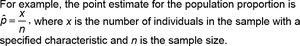
A point estimate is a single value used to approximate a population parameter. For the population proportion, the sample proportion \( \hat{p} \) is used as the point estimate:
\( \hat{p} = \frac{x}{n} \), where x is the number of individuals in the sample with the specified characteristic and n is the sample size.
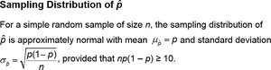
The sampling distribution of \( \hat{p} \) for a simple random sample of size n is approximately normal with mean \( \mu_{\hat{p}} = p \) and standard deviation \( \sigma_{\hat{p}} = \sqrt{\frac{p(1-p)}{n}} \), provided that \( np(1-p) \geq 10 \).
9.1.2 Construct and Interpret a Confidence Interval for the Population Proportion
A confidence interval for an unknown parameter consists of an interval of numbers based on a point estimate. For the population proportion, the confidence interval is:
\( \hat{p} \pm E \), where E is the margin of error.
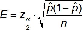
The margin of error for a confidence interval for a population proportion is:
\( E = z_{\alpha/2} \cdot \sqrt{\frac{\hat{p}(1-\hat{p})}{n}} \)

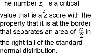
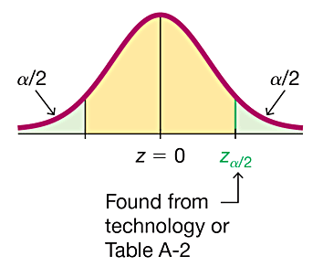
The critical value \( z_{\alpha/2} \) is the z-score that separates an area of \( \alpha/2 \) in the right tail of the standard normal distribution.
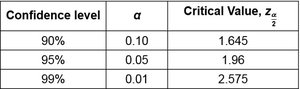
Common critical values for confidence levels are summarized below:
Confidence Level | \( \alpha \) | Critical Value, \( z_{\alpha/2} \) |
|---|---|---|
90% | 0.10 | 1.645 |
95% | 0.05 | 1.96 |
99% | 0.01 | 2.575 |
The confidence interval for the population proportion is then:
Lower bound: \( \hat{p} - z_{\alpha/2} \sqrt{\frac{\hat{p}(1-\hat{p})}{n}} \)
Upper bound: \( \hat{p} + z_{\alpha/2} \sqrt{\frac{\hat{p}(1-\hat{p})}{n}} \)
The level of confidence (e.g., 95%) represents the expected proportion of intervals that will contain the parameter if many samples are taken. The correct interpretation is: "We are 99% confident that the interval from 0.56 to 0.64 contains the true value of the population proportion p."
Example: Constructing a Confidence Interval
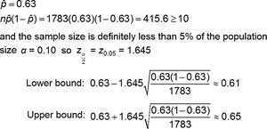
Suppose a poll of 1783 registered voters finds 1123 in favor of the death penalty. The point estimate is \( \hat{p} = 1123/1783 \approx 0.63 \). For a 90% confidence interval:
\( \alpha = 0.10 \), so \( z_{\alpha/2} = 1.645 \)
Margin of error: \( E = 1.645 \cdot \sqrt{\frac{0.63(1-0.63)}{1783}} \approx 0.02 \)
Interval: (0.61, 0.65)
9.1.3 Determine the Sample Size Necessary for Estimating a Population Proportion within a Specified Margin of Error
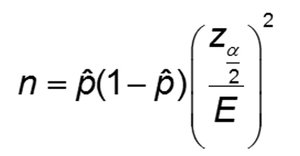
To estimate a population proportion within a specified margin of error E and confidence level, the required sample size is:
\( n = \hat{p}(1-\hat{p}) \left( \frac{z_{\alpha/2}}{E} \right)^2 \)
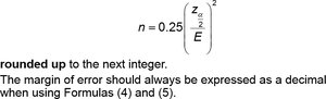
If no prior estimate of \( \hat{p} \) is available, use \( \hat{p} = 0.5 \) for the most conservative (largest) sample size:
\( n = 0.25 \left( \frac{z_{\alpha/2}}{E} \right)^2 \)
9.2 Estimating a Population Mean
9.2.1 Obtain a Point Estimate for the Population Mean
The sample mean \( \bar{x} \) is used as the point estimate for the population mean \( \mu \).
9.2.2 State Properties of Student’s t-Distribution
When the population standard deviation is unknown and the sample size is small, the Student’s t-distribution is used. The t-distribution:
Is symmetric and bell-shaped, centered at 0
Has heavier tails than the standard normal distribution
Varies with degrees of freedom (df = n - 1)
As sample size increases, approaches the standard normal distribution
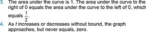
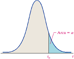
9.2.3 Determine t-Values
The notation \( t_{\alpha} \) refers to the t-value such that the area under the curve to the right is \( \alpha \), for a given number of degrees of freedom. These values are found using t-tables or statistical software.
9.2.4 Construct and Interpret a Confidence Interval for the Population Mean
For a simple random sample from a normally distributed population (or large sample size), a \( (1-\alpha) \cdot 100\% \) confidence interval for \( \mu \) is:
\( \bar{x} \pm t_{\alpha/2,\,df} \cdot \frac{s}{\sqrt{n}} \)
Where \( t_{\alpha/2,\,df} \) is the critical value from the t-distribution with df = n - 1.
Example: Estimating the Mean Weight of Pennies
Given the weights of 17 randomly selected pennies, the sample mean \( \bar{x} \) is calculated. For a 99% confidence interval, use the appropriate t-value for 16 degrees of freedom.
9.2.5 Determine the Sample Size Needed to Estimate the Population Mean within a Specified Margin of Error
The required sample size to estimate the population mean \( \mu \) with margin of error E and confidence level \( (1-\alpha) \cdot 100\% \) is:
\( n = \left( \frac{z_{\alpha/2} \cdot \sigma}{E} \right)^2 \) (if \( \sigma \) is known or approximated by s)
9.3 Putting It Together: Which Procedure Do I Use?
This section provides guidance on selecting the appropriate estimation procedure based on the parameter of interest (proportion or mean), sample size, and whether the population standard deviation is known.
Additional info: These notes are based on the structure and content of a modern statistics textbook, focusing on estimation procedures for population parameters, including point estimation, confidence intervals, and sample size determination. All formulas are provided in LaTeX format for clarity and academic rigor.
