Hypothesis Testing for One Population Mean

Introduction to Hypothesis Testing

Hypothesis testing is a fundamental statistical method used to assess the validity of a claim or statement about a population parameter, such as the mean. The process is analogous to a criminal trial, where evidence is gathered to support or refute a presumption.

• Null Hypothesis (H0): The default assumption or statement to be tested, typically involving equality.

• Alternative Hypothesis (Ha): The statement accepted if there is sufficient evidence to reject H0.

• Significance Level (α): The probability threshold (commonly 5%) for rejecting H0.

• Test Statistic: A value calculated from sample data to assess evidence against H0.

• Critical Value: The cutoff value(s) from statistical tables used to decide whether to reject H0.

Structure of a Hypothesis Test

The hypothesis testing procedure involves several key steps:

1. State the null and alternative hypotheses (H0 and Ha).

2. Choose the significance level (α), often 0.05.

3. Compute the test statistic from the sample data.

4. Determine the critical value(s) from statistical tables (z or t tables).

5. Compare the test statistic to the critical value(s) and make a decision.

Hypothesis Test for a Population Mean (Large Sample, n > 30)

Test Statistic and Decision Rule

For large samples, the test statistic follows a normal distribution and is calculated as:

• \( \bar{x} \): Sample mean

• \( \mu \): Hypothesized population mean

• \( s \): Sample standard deviation

• \( n \): Sample size

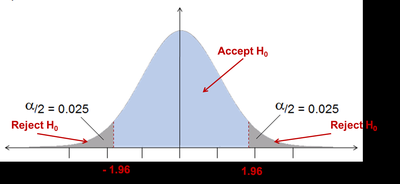
The calculated z-value is compared to critical values from the standard normal (z) table. For a two-tailed test at α = 0.05, the critical values are ±1.96.

Example: Sunday Lunch Price

• Claim: The average price of Sunday lunch in Limerick is €20.

• Sample Data: \( \bar{x} = 24.21,\ s = 5.47,\ n = 30 \)

• Hypotheses: H0: \( \mu = 20 \), Ha: \( \mu \neq 20 \)

• Test Statistic:

• Decision: Since 4.21 > 1.96, reject H0.

• Conclusion: There is evidence that the average price is not €20.

Directional and Non-Directional Tests

Hypothesis tests can be classified based on the direction of the alternative hypothesis:

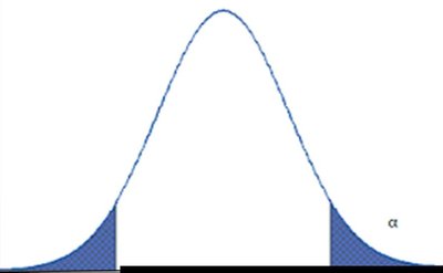
• Two-tailed (non-directional): H0: \( \mu = \mu_0 \), Ha: \( \mu \neq \mu_0 \)

• Right-tailed (directional): H0: \( \mu \leq \mu_0 \), Ha: \( \mu > \mu_0 \)

• Left-tailed (directional): H0: \( \mu \geq \mu_0 \), Ha: \( \mu < \mu_0 \)

A two-tailed test is always valid and is used when deviations in both directions are of interest.

Example: Pollution Levels

• Claim: Pollution levels in a river should be below 2.5 mg/L.

• Sample Data: \( \bar{x} = 2.37,\ s = 1.21,\ n = 72 \)

• Hypotheses: H0: \( \mu = 2.5 \), Ha: \( \mu \neq 2.5 \)

• Test Statistic:

• Decision: Since -0.91 is within ±1.96, fail to reject H0.

• Conclusion: Not enough evidence to suggest the mean pollution level is different from 2.5 mg/L.

Types of Error in Hypothesis Testing

Type I and Type II Errors

There are two types of errors that can occur in hypothesis testing:

• Type I Error (α): Rejecting H0 when it is actually true (false positive). The probability of this error is the significance level, typically 5%.

• Type II Error (β): Failing to reject H0 when it is actually false (false negative). The probability of this error is β, and 1-β is called the power of the test.

• Increasing sample size increases the power of a test.

Hypothesis Test for a Population Mean (Small Sample, n < 30)

t-Distribution and Test Statistic

When the sample size is small and the population is approximately normally distributed, the t-distribution is used:

• Degrees of freedom: \( v = n - 1 \)

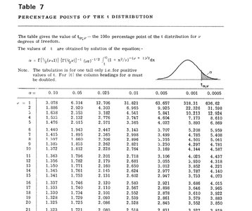
• Critical values are obtained from the t-table for the chosen significance level and degrees of freedom.

Example: Production Line Filling Weights

• Claim: Mean filling weight is 500 grams per container.

• Sample Data: \( \bar{x} = 510,\ s = 25,\ n = 20 \)

• Hypotheses: H0: \( \mu = 500 \), Ha: \( \mu \neq 500 \)

• Test Statistic:

• Critical Value: For v = 19, α = 0.025 (two-tailed), tcrit ≈ 2.093.

• Decision: Since 1.78 < 2.093, fail to reject H0.

• Conclusion: Not enough evidence to suggest the machine is overfilling.

Summary Table: Hypothesis Testing for One Mean

Key Points

• Hypothesis testing provides a structured approach to assess claims about population means.

• Large samples use the z-distribution; small samples use the t-distribution.

• Type I and Type II errors are inherent risks in hypothesis testing; significance level controls Type I error.

• Always clearly state hypotheses, significance level, test statistic, and conclusion.