Modeling Random Events: The Normal and Binomial Models

Section 6.1: Probability Distributions Are Models of Random Experiments

Probability distributions are fundamental tools in statistics for modeling the outcomes of random experiments. They describe all possible outcomes and the likelihood of each outcome occurring.

• Probability Distribution: A table or graph that lists all possible outcomes of a random experiment and the probability of each outcome.

• Discrete Random Variables: Variables that take on countable values (e.g., number of siblings).

• Continuous Random Variables: Variables that take on values over a range and cannot be listed individually (e.g., height, weight).

• Key Features:

  • All probabilities must be between 0 and 1.

  • The sum of all probabilities must equal 1.

• Probability Distribution Table Example: Rolling a die and calculating the probability of rolling a 5 or 6.

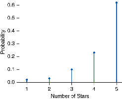
• Probability Distribution Graph Example: Estimating the probability of a reviewer giving a three-star rating.

• Probability Distributions for Continuous Variables: Represented by probability density curves, not tables.

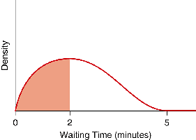
• Probability Density Curve Example: Shows the probability of wait times before service at a coffee shop. The shaded area represents the probability of a wait time between 0 and 2 minutes.

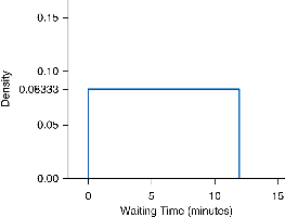
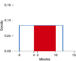
• Uniform Distribution Example: Probability distribution for bus wait times, with the probability of waiting between 4 and 10 minutes shown as the area of a rectangle.

Section 6.2: The Normal Model

The Normal model is one of the most widely used probability models for continuous numerical random variables. It is also known as the "bell curve" due to its shape.

• Normal Distribution: A symmetric, unimodal distribution used to model many natural phenomena (e.g., heights, test scores).

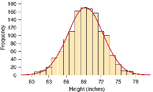
• Visualizing the Normal Model: Histogram of heights for a sample of males, showing symmetry and unimodality.

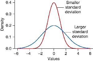
• Same Mean, Different Standard Deviation: Two Normal distributions with the same mean but different spreads.

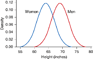
• Different Means, Same Standard Deviation: Normal curves for heights of men and women, showing different centers but similar spreads.

• Notation:

  • represents the mean.

  • represents the standard deviation.

  • denotes a Normal distribution with mean and standard deviation .

• Finding Probabilities: Use technology or tables to find areas under the Normal curve for given intervals.

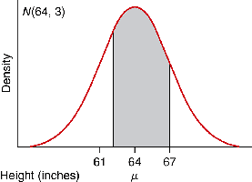
• Example: Probability of Women's Heights Between 62 and 67 Inches:

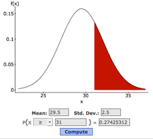
• Using StatCrunch: Example with Pacific harbor seal pups, finding probability that a pup is longer than 31 inches.

• Standard Normal Model: A Normal distribution with mean 0 and standard deviation 1.

• Z-Scores: Standard units indicating how many standard deviations an observation is from the mean.

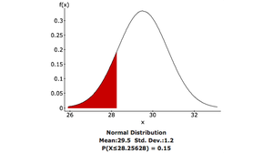
• Example: Probability of Seal Pup Length Below 28 Inches:

• Inverse Normal Problems: Finding the value corresponding to a given percentile (e.g., 15th percentile for seal pup length).

Section 6.3: The Binomial Model

The Binomial model is used for situations with discrete numerical variables, especially when there are only two possible outcomes for each trial.

• Binomial Probability Model: Applies when:

  • There is a fixed number of trials ().

  • Each trial has only two outcomes (success or failure).

  • The probability of success () is the same for each trial.

  • Trials are independent.

• Example: Tossing a Coin Eight Times: Fixed number of trials, two outcomes, constant probability, independent trials.

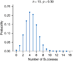
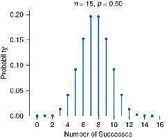
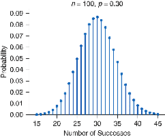
• Shape of Binomial Distribution: Depends on and . Symmetric if or if is large.

• Finding Binomial Probabilities: Use the Binomial formula or technology for larger .

  • Binomial formula:

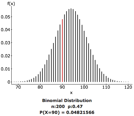
• Example: Probability Exactly 90 Out of 200 Americans Support Gun Control:

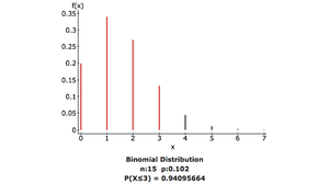
• Example: Probability Three or Fewer Unemployed in Detroit Sample:

• Language in Binomial Problems: Pay attention to phrases like "more than 5" (x > 5) vs. "5 or more" (x ≥ 5).

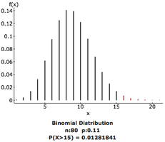
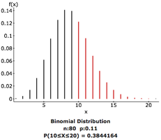
• Example: Medical Coverage in California:

  • Probability more than 15 lack insurance:

  • Probability between 10 and 20 (inclusive) lack insurance:

• Mean of a Binomial Distribution: Expected value, calculated as .

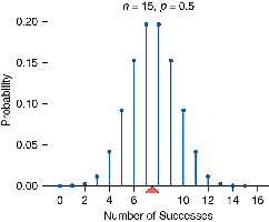
  • Example: Tossing a fair coin 15 times, expected heads = .

• Standard Deviation of a Binomial Distribution: Measures spread, calculated as .

• Example: Buster Posey Batting: Expected hits and standard deviation for 480 at-bats with batting average 0.308.

• Z-Score for Binomial Distribution:

Practice Questions

• Discrete Variable Example: Number of passengers in a car is discrete.

• Normal Model Questions:

  • Percentage of U.S. women taller than 61 inches (StatCrunch): 0.820, 0.841, 0.909, 0.914

  • Probability between 62 and 65 inches (TI Calculator): 0.340, 0.378, 0.472, 0.680

  • Standard Normal Model: Mean 0, standard deviation 1.

  • Height at 90th percentile (TI Calculator): 57.6, 67.0, 67.8, 68.7 inches

• Binomial Model Questions:

  • Characteristic NOT of binomial model: Trials are dependent.

  • Probability more than 50 unemployed in sample of 500: 0.064, 0.086, 0.124, 0.410

  • Would 50 unemployed be surprising? No, because it is only about 1.5 standard deviations below expected value.

Summary Table: Binomial vs. Normal Distributions

Additional info: Academic context and examples were expanded for clarity and completeness. Images included only when directly relevant to the explanation.