Normal Approximation to the Binomial Distribution

Introduction to Normal Approximation

The normal approximation to the binomial distribution is a statistical method used to estimate binomial probabilities when the sample size is large. This approach is particularly useful when calculating exact binomial probabilities is cumbersome. The approximation uses a normal distribution with the same mean and standard deviation as the binomial random variable.

• Mean of binomial:

• Standard deviation of binomial:

• Conditions for accuracy: The approximation is considered accurate when both and .

Example: Tossing a die 120 times, the probability of rolling a "6" 25 times or more can be approximated using the normal distribution, provided the conditions above are met.

Solving Binomial Problems with Normal Approximation

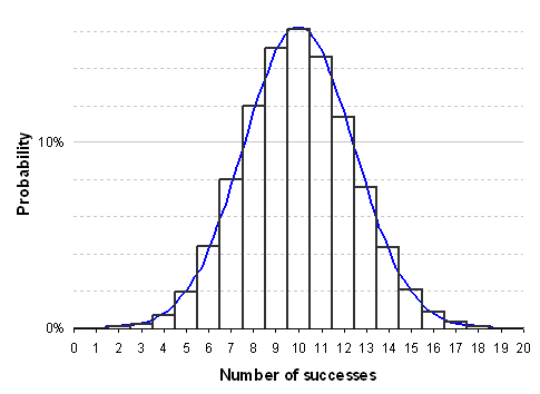
Some complex binomial probability problems can be simplified by approximating the histogram of the number of successes with a normal curve. This is especially helpful for large sample sizes.

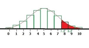
• Continuity correction: When using the normal approximation for discrete binomial variables, a continuity correction is applied. For example, to approximate , consider the interval from 7.5 to 8.5, so , where is the continuous normal random variable.

Example: If we consistently observe 30 or more "6"s in 120 die rolls, we may question whether the die is fair, using the normal approximation to assess the probability of such an outcome.

Sampling Distributions

Parameters vs. Statistics

In statistics, we often estimate unknown population parameters using sample statistics. This is necessary because populations are typically too large or inaccessible to measure directly.

• Parameter: A numerical value describing a characteristic of a population (e.g., population mean, population proportion).

• Statistic: A numerical value describing a characteristic of a sample (e.g., sample mean, sample proportion).

Example: Estimating the proportion of students unable to get summer jobs, or the mean time spent on social media, involves collecting sample data and using sample statistics to infer population parameters.

Sampling Error

The sampling error quantifies the difference between a sample statistic and the corresponding population parameter:

• Formula: Sampling error = (sample statistic) – (population parameter)

Example: In a sample of 120 cups, 12 are winners. Population proportion , sample proportion . Sampling error = .

Sampling Distribution of Sample Proportion ()

The sampling distribution of is the distribution of all possible sample proportions obtained from repeated random samples of the same size from the population.

• Mean (expected value):

• Standard deviation (standard error):

• Central Limit Theorem (CLT) for proportions: As sample size increases, the sampling distribution of approaches a normal distribution, provided and .

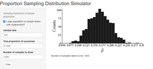
Example: Simulating the sampling distribution by visiting 1000 Tim Hortons locations and buying 120 cups at each, the histogram of sample proportions will center around the population proportion .

Summary Table: Binomial vs. Normal Approximation

Summary Table: Parameters vs. Statistics

Additional info: The act of averaging (taking sample means or proportions) leads to distributions that are approximately normal, as described by the Central Limit Theorem.