 Back
BackNormal Distribution and Sampling Distribution of Means: Study Notes
Study Guide - Smart Notes
 Tailored notes based on your materials, expanded with key definitions, examples, and context.
Normal Distribution and Sampling Distribution of Means
Probability Density Function
The probability density function (PDF) is a fundamental concept in statistics used to compute probabilities for continuous random variables. It possesses two essential properties:
Non-negativity: The graph of the PDF must lie on or above the horizontal axis.
Total Area: The area under the graph must equal 1, representing the total probability.
Example: The normal distribution is a common example of a probability density function.
Normal Distribution
The normal distribution is a continuous probability distribution characterized by its bell-shaped and symmetric curve. It is also known as the Gaussian Distribution, named after Carl Gauss, and is widely used to model natural phenomena.
Notation: Normal distributions are denoted as N(μ, σ) or N(μ, σ2), where μ is the mean and σ is the standard deviation.
Range: The variable x ranges from −∞ to +∞.
Parameters: The distribution is fully described by its mean (μ) and standard deviation (σ).
Example: N(20, 3) or N(20, 32) represents a normal distribution with mean 20 and standard deviation 3.
Features of the Normal Curve
The normal curve exhibits several important features:
Bell-shaped: The curve is highest at the mean and symmetric about a vertical line through μ.
Central tendency: The mean, median, and mode are approximately equal (μ ≅ median ≅ mode).
Asymptotic: The curve approaches but never touches the horizontal axis.
Spread: As σ increases, the curve spreads out; as σ decreases, it becomes more peaked around μ.
Example: Curves with the same mean but different standard deviations will have different spreads.
Normal Distribution Function
The mathematical formula for the normal distribution is:
Where μ is the population mean and σ is the population standard deviation.
Example: A curve with μ = 2 and σ = 0.25 is more peaked than one with μ = 3 and σ = 0.5.
Normal Probability and Area Under the Curve
The area under the normal curve within a given interval represents the probability that a measurement will fall within that interval. The total area under the curve is 1, and the data is equally distributed on each side of the mean:
50% of the data lies to the left of μ
50% of the data lies to the right of μ
Identifying Normal Data
There are several methods to determine if a dataset follows a normal distribution:
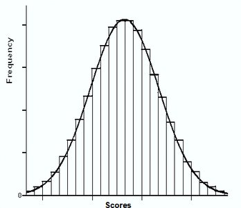
Histogram: A normal distribution's histogram should be roughly bell-shaped.
Outliers: A normal distribution should have no more than one outlier.
Quantile Plot (QQ Plot): If the data points lie close to a straight line, the data is approximately normal.
Example: The histogram below shows a bell-shaped distribution, indicating normality.
Empirical Rule (68-95-99.7 Rule)
The empirical rule describes the proportion of data within certain standard deviations of the mean in a normal distribution:
About 68% of the area is within one standard deviation (μ ± σ)
About 95% of the area is within two standard deviations (μ ± 2σ)
About 99.7% of the area is within three standard deviations (μ ± 3σ)
This rule is useful for quickly estimating probabilities and identifying outliers in normally distributed data.
