Normal Probability Distributions

Continuous Probability Distributions

Continuous probability distributions describe the probabilities of outcomes for continuous random variables. Two important types are the uniform distribution and the normal distribution. The graph of a continuous probability distribution is called a density curve, which must satisfy:

• The total area under the curve equals 1.

• Every point on the curve has a vertical height of 0 or greater (the curve cannot fall below the x-axis).

Uniform Distribution

A uniform distribution occurs when all values within a certain interval are equally likely. The density curve is rectangular, and probabilities are calculated using the area of the rectangle.

• Density function: For a uniform distribution on the interval [a, b], the probability density function is: for

• Area and Probability: Probability is found by identifying the area under the curve for the desired interval:

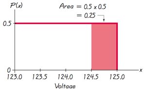
Example: Voltage Levels

Given a uniform distribution of voltage levels, the probability that a randomly selected voltage is greater than 124.5 volts is equal to the area of the shaded region.

• Height:

• Width:

• Area:

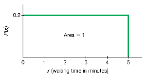
Example: Waiting Times at JFK Airport

Waiting times are uniformly distributed between 0 and 5 minutes. The probability that a passenger waits at least 2 minutes is found by calculating the area for .

Normal Distribution

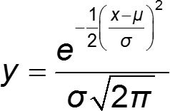
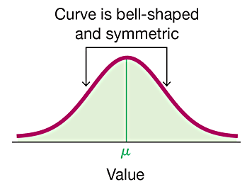
The normal distribution is a continuous probability distribution with a symmetric, bell-shaped curve. It is defined by its mean () and standard deviation ().

• Probability density function:

• The curve is symmetric about the mean.

• The total area under the curve is 1.

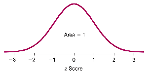
Standard Normal Distribution

The standard normal distribution is a special case of the normal distribution with and . The area under the curve is 1, and values are measured in terms of z scores.

Finding Probabilities Using z Scores

Probabilities for the standard normal distribution are found using z scores and the standard normal table (Table A-2):

• Area to the left of z: is found directly from the table.

• Area to the right of z:

• Area between two z scores:

Finding z Scores from Known Areas

To find a z score corresponding to a given probability:

1. Draw the bell-shaped curve and shade the region representing the probability.

2. Use the cumulative area from the left to locate the closest probability in the table and identify the corresponding z score.

Critical Values

A critical value is a z score that separates unlikely values from likely values. The notation denotes the z score with an area to its right.

• To find , find (area to the left).

Applications of Normal Distributions

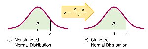
Converting to a Standard Normal Distribution

For any normal distribution (not necessarily standard), values can be converted to z scores using:

• z score formula:

Procedure for Finding Areas with a Nonstandard Normal Distribution

1. Sketch the normal curve, label the mean and relevant x values, and shade the region.

2. Convert each x value to a z score using the formula above.

3. Use the standard normal table to find the area (probability).

Sampling Distributions and Estimators

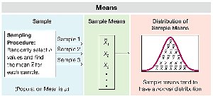
Sampling Distribution of a Statistic

The sampling distribution of a statistic (such as sample mean or proportion) is the distribution of all values of the statistic from all possible samples of the same size from a population.

• Sample means tend to be normally distributed.

• The mean of sample means equals the population mean.

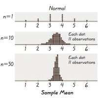
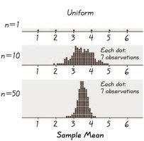
Central Limit Theorem (CLT)

The Central Limit Theorem states that for any population distribution, the distribution of sample means approaches a normal distribution as sample size increases. This is foundational for estimating population parameters and hypothesis testing.

• As sample size n increases, the distribution of sample means becomes more normal.

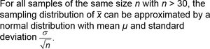
Requirements for CLT

• If the population is normal or , the sampling distribution of can be approximated by a normal distribution with mean and standard deviation .

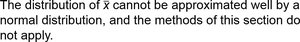
• If the population is not normal and , the distribution of cannot be approximated well by a normal distribution.

Practical Considerations

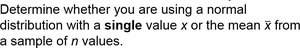
• Determine whether you are using a normal distribution for a single value x or the mean from a sample of n values.

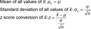
Formulas for Sampling Distributions

• Mean of all sample means:

• Standard deviation of all sample means:

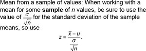
• z score conversion for sample means:

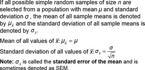
Note: is called the standard error of the mean (SEM).