Normal Probability Distributions

Standard Normal Distribution

The standard normal distribution is a special case of the normal probability distribution with a mean of 0 and a standard deviation of 1. It is widely used in statistics for calculating probabilities and z-scores.

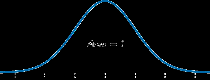
• Bell-shaped curve: The graph is symmetric and centered at zero.

• Mean (μ): 0

• Standard deviation (σ): 1

• Total area under the curve: 1 (corresponds to probability 1)

Because the total area under the curve is 1, the area under the curve between two points represents the probability of a value falling within that range.

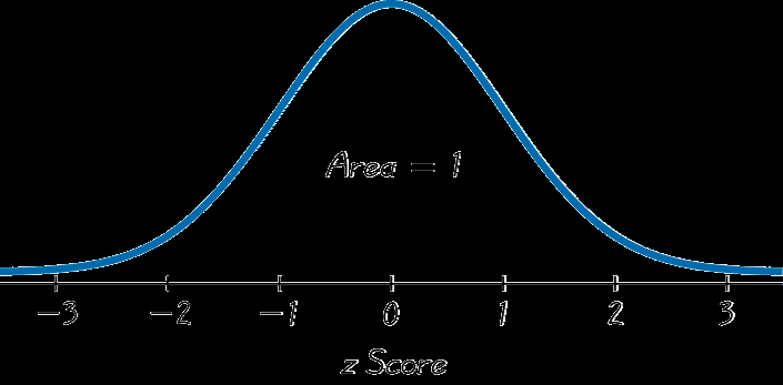
z-Scores

A z-score measures how many standard deviations a value is from the mean. Each unit on the z-scale represents one standard deviation. The formula for a z-score is:

• Unusual events: Typically, z-scores less than -2 or greater than 2 are considered unusual, but the threshold may vary depending on context.

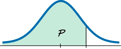
Finding Areas and Probabilities

To find the probability that a value falls within a certain range, use the area under the curve between the corresponding z-scores. Calculators and statistical tables can be used for this purpose. For example, the calculator function normalcdf(L.B., U.B., μ, σ) gives the area (probability) between two bounds.

Example: Bone Density Test

• Context: Bone density z-scores are normally distributed with μ = 0 and σ = 1.

• Find the probability of a reading less than 1.27: Use normalcdf(-∞, 1.27, 0, 1).

• Find the probability of a reading above -1.00: Use normalcdf(-1.00, ∞, 0, 1).

• Probability of osteopenia (between -1.00 and -2.50): Use normalcdf(-2.50, -1.00, 0, 1).

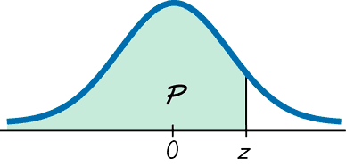
Finding Probabilities for Given z-Scores

To find the probability for a given z-score, calculate the area under the curve to the left (for less than) or to the right (for greater than) that z-score.

• Less than z = -1.50: Area to the left of -1.50

• Greater than z = 2.22: Area to the right of 2.22

• Between z = -1.20 and z = 1.95: Area between these two z-scores

Finding z-Scores for Given Probabilities

To find the z-score corresponding to a given cumulative probability (area to the left), use the InvNorm function:

• InvNorm(area, μ, σ): Returns the z-score for the specified area to the left.

Examples:

• Find the z-score for area = 0.7542

• Find the z-score for area = 0.2222

• Find the z-score for the top 40% (area to the left = 0.60)

• Find the z-score for the top 95% (area to the left = 0.05 for the lower tail, or 0.95 for the upper tail)

Applications of Normal Distributions

Standard vs. Non-Standard Normal Distributions

The standard normal distribution uses μ = 0 and σ = 1. A non-standard normal distribution has any mean μ and standard deviation σ. To use standard normal tables or calculator functions, convert values to z-scores.

Example: Tall Clubs International

• Requirement: Women must be at least 70 inches tall.

• Given: Heights are normally distributed with μ = 63.8 in, σ = 2.6 in.

• Find: Percentage of women who meet the requirement (P(X ≥ 70)).

• Solution: Convert 70 to a z-score, then use normalcdf(70, ∞, 63.8, 2.6).

Example: Water Taxi Load

• Safe load: 3500 lb; mean passenger weight = 172 lb; σ = 29 lb.

• Find: Probability a randomly selected man weighs less than 174 lb.

• Solution: Use normalcdf(-∞, 174, 172, 29).

Example: Aircraft Cabin Height

• Goal: Find ceiling height so 95% of men can stand without bumping heads.

• Given: μ = 69.5 in, σ = 2.4 in.

• Solution: Use InvNorm(0.95, 69.5, 2.4) to find the required height.

Example: Newborn Baby Weights

• Given: μ = 7 lb, σ = 2.5 lb.

• Find: The 82nd percentile (P82), the weight separating the bottom 82% from the top 18%.

• Solution: Use InvNorm(0.82, 7, 2.5).

Central Limit Theorem (CLT)

Sampling Distributions and the CLT

The Central Limit Theorem states that the distribution of sample means approaches a normal distribution as the sample size increases, regardless of the population's distribution, provided the samples are independent and identically distributed.

• Mean of sample means: μx̄ = μ

• Standard deviation of sample means (standard error):

The z-score formula for sample means is:

To find probabilities for sample means, use normalcdf(L.B., U.B., μ, σ/√n).

Example: Water Taxi with 25 Passengers

• Safe load: 3500 lb; mean passenger weight = 172 lb; σ = 29 lb; n = 25.

• Find: Probability that the mean weight of 25 men exceeds 175 lb.

• Solution: Use the CLT formula for z, then normalcdf(175, ∞, 172, 29/√25).

Example: Elevator Capacity

• Maximum capacity: 16 passengers, 2500 lb total; mean male weight = 182.9 lb; σ = 40.8 lb.

• a. Probability one male exceeds 156.25 lb: Use normalcdf(156.25, ∞, 182.9, 40.8).

• b. Probability mean of 16 males exceeds 156.25 lb: Use normalcdf(156.25, ∞, 182.9, 40.8/√16).

Summary Table: Key Normal Distribution Functions