Normal Probability Distributions

Introduction to Normal Distributions

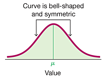
The normal distribution is a fundamental concept in statistics, describing how data values are distributed in many natural and social phenomena. It is characterized by its bell-shaped, symmetric curve and is widely used for probability calculations and inferential statistics.

• Normal Distribution: A continuous probability distribution that is symmetric about the mean, showing that data near the mean are more frequent in occurrence than data far from the mean.

• Standard Normal Distribution: A special case of the normal distribution with a mean (μ) of 0 and a standard deviation (σ) of 1.

• Density Curve: The graph of a continuous probability distribution, where the total area under the curve is exactly 1.

Relationship Between Probability and Area

For continuous probability distributions, the probability of an event corresponds to the area under the curve over the interval representing the event. For example, the probability that a randomly selected value falls within a certain range is equal to the area under the curve for that range.

• Key Principle: Probability = Area under the density curve for the specified interval.

• Example: If a satellite crashes randomly on Earth, the probability it lands on land is the area of land divided by the total area of Earth.

Uniform Distribution

Definition and Properties

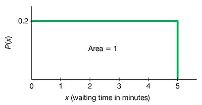
A uniform distribution is a type of continuous probability distribution where all outcomes are equally likely within a certain interval. Its graph is a rectangle, and the area under the curve is always 1.

• Property 1: The area under the graph is 1.

• Property 2: Probabilities are found by calculating the area of the rectangle:

• Uniform Distribution: All values within the range are equally likely.

Example: Waiting Times for Airport Security

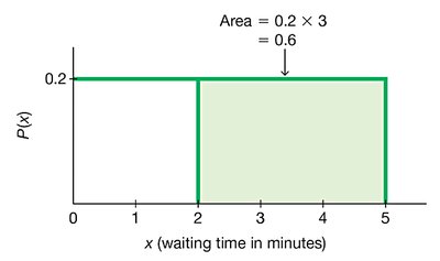
Suppose waiting times at an airport security checkpoint are uniformly distributed between 0 and 5 minutes. The probability that a randomly selected passenger waits at least 2 minutes can be found by calculating the area under the curve from 2 to 5 minutes.

• Step 1: The height of the rectangle is (since ).

• Step 2: The width for waiting at least 2 minutes is minutes.

• Step 3: Probability =

The Standard Normal Distribution

Definition and Properties

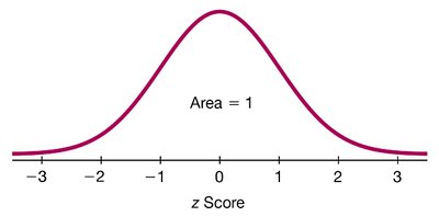
The standard normal distribution is a normal distribution with a mean of 0 and a standard deviation of 1. It is used as a reference to find probabilities and percentiles for any normal distribution by converting values to z scores.

• Mean (μ): 0

• Standard Deviation (σ): 1

• Total Area: 1

z Scores

A z score indicates how many standard deviations a value is from the mean. It is calculated as:

• z score: Distance along the horizontal axis of the standard normal distribution.

• Area: Region under the curve corresponding to a probability.

Finding Probabilities Using z Scores

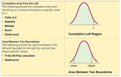
To find probabilities for normal distributions, use technology (such as Excel or calculators) or statistical tables (Table A-2). The area under the curve to the left of a z score gives the cumulative probability.

• Table A-2: Provides cumulative areas from the left for standard normal z scores.

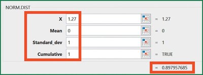
• Technology: Functions like NORM.DIST in Excel can be used for more accurate results.

Example: Bone Density Test

Suppose bone density test results are normally distributed with a mean of 0 and a standard deviation of 1. To find the probability that a randomly selected person has a test score less than 1.27:

• Step 1: Find the area to the left of z = 1.27 using Table A-2 or Excel.

• Step 2: The cumulative area is approximately 0.8980.

• Interpretation: 89.80% of people have bone density levels below 1.27.

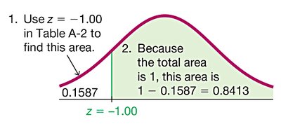
Finding the Area to the Right of a Value

To find the probability that a value is greater than a given z score, subtract the cumulative area to the left from 1.

• Example: Probability of a bone density reading above z = -1.00:

• Cumulative area to the left: 0.1587

• Area to the right:

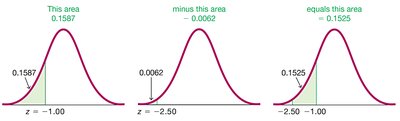
Finding the Area Between Two Values

To find the probability that a value falls between two z scores, subtract the cumulative area to the left of the lower z score from the cumulative area to the left of the higher z score.

• Example: Probability that a bone density reading is between z = -2.50 and z = -1.00:

• Area to the left of z = -1.00: 0.1587

• Area to the left of z = -2.50: 0.0062

• Area between:

Notation for Probabilities

• P(a < z < b): Probability that z is between a and b.

• P(z > a): Probability that z is greater than a.

• P(z < a): Probability that z is less than a.

Finding z Scores from Known Areas

Given a probability (area), you can find the corresponding z score using statistical tables or technology. For example, the z score for the 95th percentile (area = 0.95 to the left) is approximately 1.645.

• Excel Function: =NORM.INV(0.95, 0, 1)

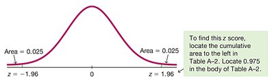
• Table A-2: Find the closest area in the body of the table and read the corresponding z score.

Critical Values

A critical value is a z score that separates significantly low or high values from the rest of the distribution. The notation zα denotes the z score with an area of α to its right.

• To find zα: Use the cumulative area to the left (1 - α) in tables or technology.

• Example: z0.025 is the z score with 0.025 area to its right (or 0.975 to its left), which is 1.96.

Additional info: Understanding the relationship between area and probability is essential for interpreting results from normal distributions and for conducting hypothesis tests and confidence intervals in later chapters.