 Back
Back5.1 Probability Distributions: Discrete Random Variables and Their Properties
Study Guide - Smart Notes
 Tailored notes based on your materials, expanded with key definitions, examples, and context.
Probability Distributions
Definition of Probability
Probability is the measure of the likelihood that a particular event will occur. It is not a guarantee of occurrence, but rather a quantification of uncertainty. For example, a 20% chance of rain does not ensure rain, nor does it ensure dryness; most events have probabilities between 0 and 1, not exactly 0 or 1.
Probability is always a value between 0 (impossible event) and 1 (certain event).
Probabilities are used to describe the uncertainty of outcomes in random experiments.
Key Concepts in Probability Distributions
This section introduces the concepts of random variables and probability distributions, including how to visualize them and calculate their key parameters.
Random Variable: A variable (usually denoted by x) that takes on numerical values determined by the outcome of a random process.
Probability Distribution: A function, table, or graph that assigns probabilities to each possible value of a random variable.
Probability Histogram: A graphical representation of a probability distribution, where the vertical axis shows probabilities.
Parameters: The mean, variance, and standard deviation of a probability distribution describe its central tendency and spread.
Significant outcomes can be identified using statistical rules, such as the range rule of thumb.
Types of Random Variables
Discrete Random Variables
A discrete random variable has a finite or countable set of possible values. For example, the number of heads in a series of coin tosses is discrete because you can count the outcomes.
Examples: Number of students in a class, number of defective items in a batch.
Continuous Random Variables
A continuous random variable can take on infinitely many values, which are not countable. These values are measured on a continuous scale, such as height or temperature.
Examples: Body temperature, time taken to run a race.
Requirements for a Probability Distribution
Every probability distribution must satisfy the following requirements:
The random variable x must be numerical, not categorical.
The sum of all probabilities must be 1: (allowing for rounding errors such as 0.999 or 1.001).
Each probability must be between 0 and 1, inclusive: for every x.
Example: Valid Probability Distribution
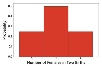
Consider the random variable x = number of females in two births. The probability distribution is:
x: Number of Females | P(x) |
|---|---|
0 | 0.25 |
1 | 0.50 |
2 | 0.25 |
x is numerical and discrete.
The probabilities sum to 1: 0.25 + 0.50 + 0.25 = 1.
Each probability is between 0 and 1.
Example: Invalid Probability Distribution
A table listing countries and the proportion of unlicensed software does not form a probability distribution because:
The variable (country) is categorical, not numerical.
The probabilities sum to more than 1 (2.09).
Probability Histograms
A probability histogram visually represents a probability distribution. The horizontal axis shows the values of the random variable, and the vertical axis shows the probability of each value. This is similar to a relative frequency histogram, but it is based on theoretical probabilities rather than sample data.
Parameters of a Probability Distribution
Population Parameters
For a probability distribution, the mean, variance, and standard deviation are parameters (since they describe the entire population, not just a sample).
Mean (μ): (the mean equals to the sum of all the values of x times their possibilities) (mean = expected value)
Variance (σ²): (easier to understand) or (easier for calculations)
Standard Deviation (σ): or Standard Deviation = (std is the square root of variance)
Expected Value
The expected value (E) of a discrete random variable is the mean of its probability distribution: . This concept is widely used in decision theory.
Example: Calculating Mean, Variance, and Standard Deviation
Given the probability distribution for the number of females in two births:
x | P(x) | x·P(x) | (x−μ)²·P(x) |
|---|---|---|---|
0 | 0.25 | 0.00 | 0.25 |
1 | 0.50 | 0.50 | 0.00 |
2 | 0.25 | 0.50 | 0.25 |
Total | 1.00 | 1.00 | 0.50 |
Mean:
Variance:
Standard deviation: (rounded)
Interpretation: In two births, the expected number of females is 1.0, with a variance of 0.5 and a standard deviation of 0.7.
Identifying Significant Results
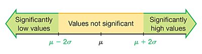
Range Rule of Thumb
The range rule of thumb helps identify significantly low or high values in a probability distribution:
Significantly low values: or lower mean - 2(standard deviation)
Significantly high values: or higher
Values not significant: Between and
Example: Using the Range Rule of Thumb
For two births, with and :
Significantly high: or more
2 females is not significantly high, since 2 < 2.4
Identifying Significant Results with Probabilities
Significantly high number of successes: x is significantly high if
Significantly low number of successes: x is significantly low if
The threshold 0.05 is common but not absolute; sometimes 0.01 is used.
The Rare Event Rule for Inferential Statistics
If, under a given assumption, the probability of an observed outcome is very small, and the outcome is significantly less or more than expected, we conclude the assumption is likely incorrect. For example, if the probability of 20 girls in 100 births is extremely low, we would question the assumption that boys and girls are equally likely.
