Sampling Distributions and Statistical Inference

Introduction to Statistical Inference

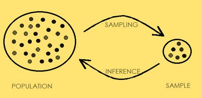
Statistical inference is the process of drawing conclusions about an entire population based on information obtained from a sample. Inferential statistics use probability theory to estimate the likelihood that a particular sample represents the population, allowing us to make informed decisions and predictions.

• Inference: A deduction or conclusion about a population based on sample data.

• Sampling: The process of selecting a subset (sample) from a larger group (population).

• Key Techniques:

  • Estimation: Includes point and interval estimates of population parameters.

  • Hypothesis Testing: Procedures for testing claims about population parameters using sample data.

  • Regression: Prediction or forecasting (not covered in this course).

Sampling Distributions

Definition and Importance

A sampling distribution is the probability distribution of a sample statistic (such as the mean or proportion) based on all possible simple random samples of the same size from the same population. Understanding sampling distributions is crucial for making valid inferences about populations.

• Focus in this course: Sampling distributions of sample means (\( \bar{x} \)) and sample proportions (\( \hat{p} \)).

Sampling Distribution of the Mean

The sample mean (\( \bar{X} \)) is a random variable whose distribution, when taken over all possible samples of size \( n \), is called the sampling distribution of the mean. This distribution has important properties that allow us to make inferences about the population mean (\( \mu \)).

• Mean of the sampling distribution: \( \mu_{\bar{X}} = \mu \)

• Standard deviation (Standard Error): \( \sigma_{\bar{X}} = \frac{\sigma}{\sqrt{n}} \)

Central Limit Theorem (CLT)

The Central Limit Theorem is a fundamental result in statistics. It states that, regardless of the population's distribution, the sampling distribution of the sample mean approaches a normal distribution as the sample size increases.

• If the population distribution is normal, the sampling distribution of the mean is also normal for any sample size.

• If the population distribution is not normal, the sampling distribution of the mean becomes approximately normal when \( n \geq 30 \) (for symmetric distributions) or larger for highly skewed distributions.

• Formula for the standard error of the mean:

Z-Formula for Sampling Distribution of Means

To standardize the sample mean and relate it to the standard normal distribution, we use the following z-score formula:

• This formula allows us to calculate probabilities and percentiles for sample means using the standard normal table.

Example: Probability Calculations for Sample Means

Suppose the time a person spends in the shower is normally distributed with mean \( \mu = 12.5 \) minutes and standard deviation \( \sigma = 3.5 \) minutes. Calculate probabilities for different sample sizes:

• For n = 1:

• For n = 25:

• For n = 121:

• For n = 9 (mean greater than 15.2):

Sampling Distribution of Proportions

Definition and Properties

Sample proportions (\( \hat{p} \)) from different surveys will vary, but as the sample size increases, the sampling distribution of \( \hat{p} \) becomes approximately normal. The mean and standard deviation of this distribution are:

• Mean:

• Standard deviation (Standard Error):

This allows us to make probability statements about sample proportions in large samples.