Chapter 8: Sampling Distributions

8.1 Distribution of the Sample Mean

The sampling distribution of the sample mean is a foundational concept in inferential statistics. It describes the probability distribution of all possible values of the sample mean computed from random samples of a fixed size drawn from a population.

Definition and Key Concepts

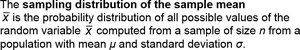
• Sampling Distribution of the Sample Mean (\( \overline{X} \)): The probability distribution of all possible values of \( \overline{X} \) computed from samples of size \( n \) from a population with mean \( \mu \) and standard deviation \( \sigma \).

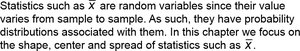
• Random Variable: Statistics such as \( \overline{X} \) are random variables because their values vary from sample to sample.

• Shape, Center, and Spread: The sampling distribution is characterized by its shape, center (mean), and spread (standard deviation).

Illustrating Sampling Distributions

• Obtain a simple random sample of size \( n \).

• Compute the sample mean.

• Repeat for all possible samples to form the sampling distribution.

Describing the Distribution: Normal Population

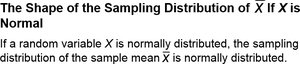
• If the population is normally distributed, the sampling distribution of \( \overline{X} \) is also normal for any sample size \( n \).

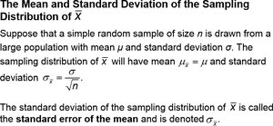
• The mean of the sampling distribution equals the population mean: \( \mu_{\overline{X}} = \mu \).

• The standard deviation (standard error) is \( \sigma_{\overline{X}} = \frac{\sigma}{\sqrt{n}} \).

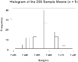
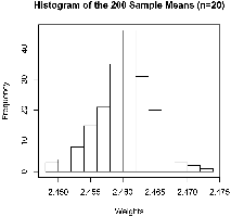
Example: Weights of Pennies

• Population: Mean \( \mu = 2.46 \) grams, Standard deviation \( \sigma = 0.02 \) grams.

• Sample size \( n = 5 \): Mean of sample means = 2.46, Standard deviation = 0.0086.

• Sample size \( n = 20 \): Mean of sample means = 2.46, Standard deviation = 0.0045.

• As \( n \) increases, the spread of the sampling distribution decreases.

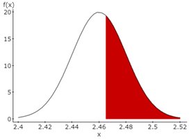
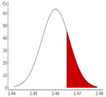
Probability Calculations with the Sample Mean

• To find probabilities involving the sample mean, use the normal distribution with mean \( \mu \) and standard error \( \sigma/\sqrt{n} \).

• Example: Probability that a sample mean is at least a certain value can be found using the standard normal (Z) transformation.

The Central Limit Theorem (CLT)

• Central Limit Theorem: For any population with mean \( \mu \) and standard deviation \( \sigma \), the sampling distribution of \( \overline{X} \) becomes approximately normal as \( n \) increases, regardless of the population's shape.

• For most practical purposes, \( n \geq 30 \) is sufficient for the sampling distribution to be approximately normal.

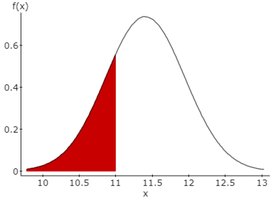
Example: Oil Change Times

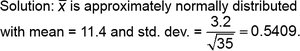
• Population: Mean = 11.4 minutes, Standard deviation = 3.2 minutes.

• Sample size \( n = 35 \): Sampling distribution of \( \overline{X} \) is approximately normal with mean 11.4 and standard deviation 0.5409.

8.2 Distribution of the Sample Proportion

The sampling distribution of the sample proportion describes the probability distribution of all possible values of the sample proportion computed from random samples of a fixed size from a population.

Definition and Key Concepts

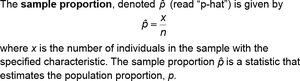
• Sample Proportion (\( \hat{p} \)): \( \hat{p} = \frac{x}{n} \), where \( x \) is the number of individuals in the sample with the specified characteristic.

• \( \hat{p} \) estimates the population proportion \( p \).

Shape, Center, and Spread of the Sampling Distribution

• The shape of the sampling distribution of \( \hat{p} \) is approximately normal if \( np(1-p) \geq 10 \).

• The mean of the sampling distribution is \( \mu_{\hat{p}} = p \).

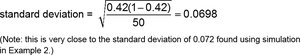
• The standard deviation is \( \sigma_{\hat{p}} = \sqrt{\frac{p(1-p)}{n}} \).

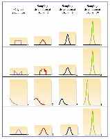
Example: Proportion of Voters

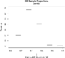
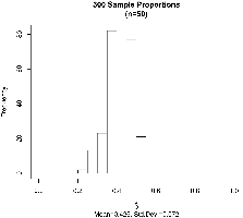
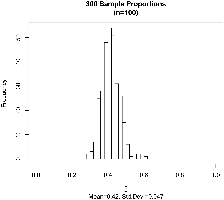
• Population proportion \( p = 0.42 \).

• Sample sizes: \( n = 10, 50, 100 \).

• As \( n \) increases, the sampling distribution becomes more normal and less spread out.

Conditions for Normality

• Sampled values must be independent (usually satisfied if sample size is less than 5% of the population).

• \( np(1-p) \geq 10 \) for approximate normality.

Probability Calculations with Sample Proportions

• To find probabilities involving \( \hat{p} \), use the normal distribution with mean \( p \) and standard deviation \( \sqrt{\frac{p(1-p)}{n}} \).

• Convert to a standard normal (Z) score for probability calculations.

Example: Overweight Children

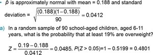
• Population proportion \( p = 0.188 \), sample size \( n = 90 \).

• Standard deviation: \( \sqrt{\frac{0.188(1-0.188)}{90}} = 0.0412 \).

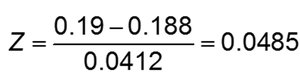
• Probability at least 19% are overweight: \( Z = \frac{0.19 - 0.188}{0.0412} = 0.0485 \).

• Probability \( P(Z > 0.05) = 0.4801 \).

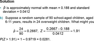
• Probability of observing 24 or more overweight children (\( \hat{p} = 0.2667 \)): \( Z = 1.91 \), \( P(Z > 1.91) = 0.0281 \).

Summary Table: Sampling Distributions

Additional info: The Central Limit Theorem is a cornerstone of inferential statistics, allowing for normal approximation in many practical scenarios. The standard error quantifies the expected variability of a statistic from sample to sample, and is crucial for constructing confidence intervals and conducting hypothesis tests.