Sampling Data

Key Concepts in Data Gathering

Sampling is fundamental in statistics, allowing researchers to draw conclusions about populations based on subsets called samples. Understanding the terminology and methods is essential for designing valid studies.

• Population: The entire set of units of interest in a study.

• Sample: A subset of units selected from the population.

• Parameter: A numerical characteristic describing the population (e.g., population mean).

• Statistic: A numerical characteristic describing the sample (e.g., sample mean).

• Response Variable: The variable of interest measured in a study.

• Explanatory Variable: A variable that explains changes in the response variable.

• Observational Study: Researchers do not impose conditions; they observe naturally occurring variables.

• Experiment: Researchers impose conditions to study effects.

• Lurking Variable: An unmeasured variable that may influence the interpretation of results.

• Confounding: Occurs when it is impossible to distinguish the effects of two variables on the response variable.

Sampling Methods

• Simple Random Sampling: Every possible sample of a given size has the same chance of being selected.

• Stratified Random Sampling: Population is divided into subgroups (strata), and random samples are taken from each.

• Voluntary Response Sampling: Individuals choose whether to participate.

• Convenience Sampling: Units are selected because they are easily accessible.

Descriptive Statistics

Types of Variables

Variables are classified as categorical or quantitative, affecting how data is summarized and analyzed.

• Categorical (Qualitative) Variable: Falls into one of two or more categories (e.g., blood type).

• Quantitative Variable: Numeric and measurable.

• Frequency: Number of observations in a category.

• Relative Frequency: Proportion of observations in a category:

• Percent Relative Frequency: Relative frequency expressed as a percentage.

• Cumulative Frequency: Number of observations in a class and all lower classes.

• Cumulative Relative Frequency:

Distribution Characteristics

Descriptive statistics summarize data distributions using measures of center, spread, and shape.

• Center: Mean and median.

• Outliers: Observations far from the overall pattern.

• Variability: Variance and standard deviation.

• Shape: Symmetry, skewness, modality.

Numerical Summaries

• Sample Mean:

• Median: Middle value when ordered; for even n, average of two middle values.

• Mode: Most frequently occurring value.

• Range:

• Mean Absolute Distance (MAD):

• Sample Variance:

• Standard Deviation:

Empirical Rule

For mound-shaped (normal) distributions:

• ~68% of observations lie within 1 standard deviation of the mean.

• ~95% within 2 standard deviations.

• ~99.7% within 3 standard deviations.

z-Score

• z-Score: Measures how many standard deviations an observation is from the mean:

Percentiles and Quartiles

• Percentile: The kth percentile is the value such that k% of ordered data values are less than or equal to it.

• Quartiles: Q1 = 25th percentile, Q2 = median, Q3 = 75th percentile.

• Interquartile Range (IQR):

• Five-number summary: Min, Q1, Median, Q3, Max.

Linear Transformation

• For , the mean of the transformed variable is

Probability

Basic Concepts

Probability quantifies uncertainty in experiments and is foundational for inferential statistics.

• Sample Space (S): Set of all possible outcomes.

• Sample Points: Individual outcomes in the sample space.

• Event: Subset of the sample space.

• Discrete: Sample points are countable.

• Continuous: Sample points form a continuum.

Rules of Probability

• For any event A:

• For any sample space S:

• Intersection (A ∩ B): Both A and B occur. If mutually exclusive,

• Union (A ∪ B): Either A, B, or both occur.

• Complement (Ac): Event A does not occur. ;

• Conditional Probability: (provided )

• Independence: Events A and B are independent if

Counting Principles

• Permutation: Ordering of a set of items; order matters.

• Combination: Selection of items; order does not matter.

R Commands for Statistics

Basic Data Analysis in R

• Enter data: data <- c(1,2,3)

• Mean: mean(data)

• Median: median(data)

• Mode: mode(data)

• Sample variance: var(data)

• Standard deviation: sd(data)

• Five-number summary: summary(data)

• Percentiles: quantile(data, p=.k, type=x)

• Permutations: factorial(#)

• Permutations (order matters): factorial(n)/factorial(n-x)

• Combinations: choose(n, x)

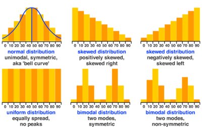
Distribution Shapes

Common Distribution Types

Understanding the shape of a distribution is crucial for selecting appropriate statistical methods and interpreting data.

• Normal Distribution: Unimodal, symmetric, bell-shaped.

• Skewed Distribution: Can be positively (right) or negatively (left) skewed.

• Uniform Distribution: Equally spread, no peaks.

• Bimodal Distribution: Two modes, can be symmetric or non-symmetric.

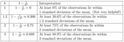
Chebyshev's Theorem

Interpretation of Chebyshev's Inequality

Chebyshev's theorem provides bounds for the proportion of observations within k standard deviations of the mean, applicable to any distribution.

Additional info:

• Some R commands and formulas are inferred for completeness and clarity.

• Distribution shapes and Chebyshev's theorem are visually supported by included images.