Chapter 7: The Normal and Other Continuous Distributions

7.1 The Standard Deviation as a Ruler

The standard deviation provides a universal scale for comparing values from different distributions. By converting values to z-scores, we can determine how many standard deviations a value is from the mean, allowing for standardized comparisons.

• Z-score: The number of standard deviations a value is from the mean. Calculated as .

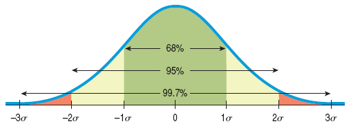
• 68-95-99.7 Rule: In a unimodal, symmetric (Normal) distribution:

  • About 68% of values fall within 1 standard deviation of the mean.

  • About 95% within 2 standard deviations.

  • About 99.7% within 3 standard deviations.

• Example: A Dow Jones drop of 634.8 points with a mean daily change of 1.87 and standard deviation of 155.28 yields a z-score of approximately , an extremely rare event (probability < 0.0015).

7.2 The Normal Distribution

The Normal distribution is a model for symmetric, bell-shaped, unimodal data. It is denoted as , where is the mean and is the standard deviation. The standard Normal distribution is , used for standardized z-scores.

• Finding Normal Percentiles: Use the 68-95-99.7 Rule for integer z-scores, or consult Normal tables/technology for other values.

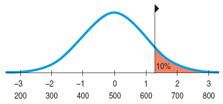
• Example 1: SAT scores are . A score of 600 is 1 SD above the mean; about 16% of students score higher.

• Example 2: Proportion of SAT scores between 450 and 600:

  • For 600: ; for 450:

  • Area between: (53.3%)

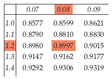
• Working Backwards: To find the score corresponding to a percentile, use the Normal table to find the z-score, then convert back to the original scale.

• Example 3: Top 10% SAT cutoff (90th percentile): , so cutoff = (rounded to 630).

• Application Example: Tire Company

  • Tread life is miles.

  • Probability a tire lasts >40,000 miles: ; probability is about 0.7%.

  • To guarantee for no more than 1 out of 25 customers (4%), find the 4th percentile: , so guarantee = (rounded to 27,000 miles).

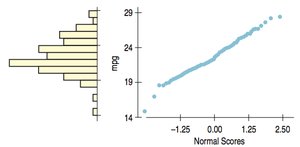
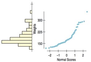
7.3 Normal Probability Plots

A Normal probability plot helps assess whether data are approximately Normal. If the plot is roughly a straight line, the data are likely Normal. Deviations from linearity indicate skewness or outliers.

• Example: Gas mileage data for a Nissan Maxima is nearly Normal; men's weights show skewness.

7.4 The Distribution of Sums of Normals

The sum or difference of independent Normal random variables is also Normal. The mean of the sum is the sum of the means, and the variance of the sum is the sum of the variances.

• Formulas:

  • Mean:

  • Variance: (if independent)

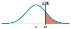
• Example: Packing two stereo systems, each with mean 9 min, SD 1.5 min:

  • Total mean: $18\sqrt{1.5^2 + 1.5^2} = 2.12$ min

  • Probability total time > 20 min: Find ; area to the right is about 17%.

7.5 The Normal Approximation for the Binomial

When the number of trials is large and both and are at least 10, the Binomial distribution can be approximated by a Normal distribution:

• Mean:

• Standard deviation:

• Example: Probability of finding a prize in a cereal box is 20%. For 50 boxes, , ; the distribution is nearly Normal.

7.6 Other Continuous Random Variables

Besides the Normal, other continuous distributions are used in statistics. Two common examples are the Uniform and Exponential distributions.

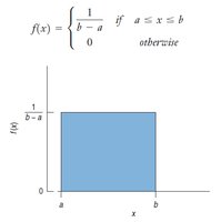
The Uniform Distribution

The Uniform distribution models outcomes equally likely over an interval . The probability density function is:

• Mean:

• Variance:

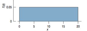
• Example: Waiting time for a bus arriving every 20 minutes is Uniform(0, 20).

Summary of Key Points

• Check for Normality using histograms and Normal probability plots.

• Use z-scores and the 68-95-99.7 Rule to judge extremity of values.

• Use Normal tables or technology for probability calculations.

• The sum/difference of independent Normals is Normal; add means and variances.

• Other continuous models (Uniform, Exponential) are used when appropriate.

• Probability models are simplifications; always check assumptions before applying them.