In Exercises 21 and 22, (a) identify the claim and state H₀ an...

Question

In Exercises 21 and 22, (a) identify the claim and state H₀ and Hₐ, (b) find the critical value and identify the rejection region, (c) find the test statistic F, (d) decide whether to reject or fail to reject the null hypothesis, and (e) interpret the decision in the context of the original claim. Assume the samples are random and independent, the populations are normally distributed, and the population variances are equal.

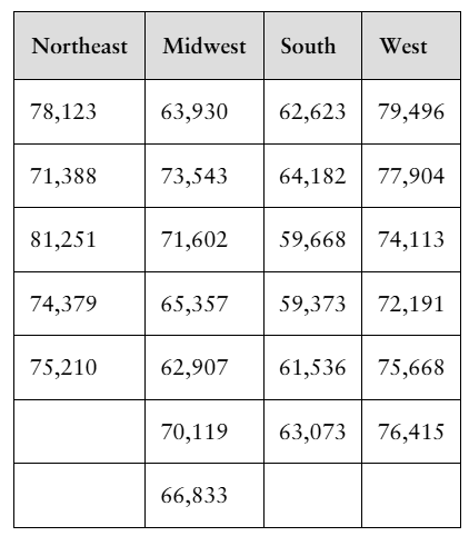
[APPLET] The table shows the annual incomes (in dollars) for a sample of families from four regions of the United States. At α=0.05, can you conclude that the mean annual income of families is different in at least one of the regions? (Adapted from U.S. Census Bureau)

Accepted Answer

Hi everybody and welcome back. Our next question says. A sociologist wants to determine whether there is a significant difference in the average number of weekly work hours among employees in 4 different industries technology, healthcare, education, and manufacturing. A sample of 28 employees is taken, and a one way a Nova is conducted. The results are as followed. Our number of groups or industries is 4, total sample size is 28. The sum of squares between or SSB is 1,482.6, and the sum of squares within or SSW is 2,654.8. At a significance level of alpha equals 0.05. Can the sociologist conclude that there is a difference in mean weekly work hours among the industries? Yes, because the F statistic is greater than the critical value. Be no, because the F statistic is less than the critical value. C, yes, because SSB is greater than SSW, or D, no, because the sample size is too small to draw any conclusion. We can go ahead and eliminate choice D because 28 is not too small a sample size. And we need to think about what we need to analyze this and determine if there's a difference in mean weekly work hours. And for that, we want the test statistic. To compare to the critical value. And in the case of multiple groups and they're mean, we're looking at the F statistic. And the F critical value. So, we're going to be looking at A or B, not choice C. So SSB and SSW go into calculating. That critical value. But will not give us our answers, so we'll say not. Sufficient So let's think about what we need to calculate our F statistic. So we recall that F. Is equal to the mean square between samples or MS sub B. In the numerator divided by the mean of squares. Within or MSWW. And we'll also need degrees of freedom, and recall that we have a um degrees of freedom for the numerator and degrees of freedom for the denominator. So for the numerator. We have the degrees of freedom between. equal to K minus 1. Where K is the number of groups. So we have 4 groups, so, K minus 1 is equal to 3. And then for the denominator are degrees of freedom or degrees of freedom within. R equal to N minus K, meaning the total sample size minus the number of groups. So, that's 28 minus 4. Which equals 24. So there's our degrees of freedom that we'll need. And now we need to go through with calculating that test statistic. Well, we don't have the mean. Square values, but we can obtain them from the values we have for the sum of squares. So, we have the sum of squares both between and within from our Enova test. So let's go ahead and calculate for the Mean of squares between MS B, that's going to equal the sum of squares between divided by the degrees of freedom between. So, that SSB value was 1,482.6. And our degrees of freedom between are 3, so 1,482.6 divided by 3. And that's going to equal 494.2. Then our mean square within would be our sum of squares within SSW divided by our degrees of freedom within. So our SSW value in the numerator will be 2,654.8. Divided by that DF subW, which is 24. That's going to equal approximately 110.62. So, now we have what we need to calculate our F. Value, so that equals the mean square between, which is 494.2, divided by the mean squares within, which is 110.62. And that's going to give us an F value of approximately 4.47. So now we need to compare that to our critical F value, which we'll get from a table. So R F Critical We're going to need. Alpha, which we're told is 0.05. And then we'll need our degrees of freedom again. So, here's where we want to recall for looking up at the table, that our degrees of freedom with between our the degrees of freedom of our numerator, so that equals 3, and the degrees of freedom of our denominator. Which equals 24, just because that's how they're usually described in those tables. So, when we use our table for 0.05, and then look up with our two degrees of freedom, we're going to get that our critical F value is approximately 3.01. So, let's compare that. We have this F of 4.47. That is greater than 3.01. Which are critical. So that means we can reject. They know hypothesis. Recall that when we're looking at one way a no results, we're talking about a right-tailed comparison there. So recall that whenever we're doing Enova or null hypothesis. Is that all the means? are equal. So, if we reject that null hypothesis, our answer will, since our question is, is there a difference in mean weekly work hours among the industries? Our answer is choice A, yes, because the F statistic is greater than the critical value. So, again, we used our AOA data to determine whether there was a significant difference in the average number of weekly work hours. We were given the number of groups, our total sample size, and then the sum of squares between and within. With an alpha equals 0.05. So, that allowed us to calculate our F test test statistic, and that's a tongue twister, and to compare it to our critical F value, and our answer is, choice A, yes, we can conclude there's a difference, because the F statistic is greater than the critical value. See you in the next video.

Key Concepts

Hypothesis Testing

ANOVA (Analysis of Variance)

Critical Value and Rejection Region

Watch next