Textbook Question
Using properties of integrals Use the value of the first integral I to evaluate the two given integrals.
I = ∫₀¹ (𝓍³ ― 2𝓍) d𝓍 = ―3/4
(a) ∫₀¹ (4𝓍―2𝓍³) d𝓍
110
views
 Verified step by step guidance
 06:11
06:11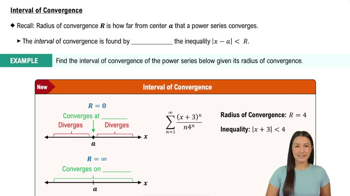 08:44
08:44 4:26
4:26Using properties of integrals Use the value of the first integral I to evaluate the two given integrals.
I = ∫₀¹ (𝓍³ ― 2𝓍) d𝓍 = ―3/4
(a) ∫₀¹ (4𝓍―2𝓍³) d𝓍
Area functions for linear functions Consider the following functions ƒ and real numbers a (see figure).
(a) Find and graph the area function A (𝓍) = ∫ₐˣ ƒ(t) dt .
ƒ(t) = 2t + 5 , a = 0
{Use of Tech} Approximating definite integrals with a calculator Consider the following definite integrals.
(a) Write the left and right Riemann sums in sigma notation for an arbitrary value of n.
∫₀¹ cos ⁻¹ 𝓍 d𝓍
Average value with a parameter Consider the function ƒ(𝓍) = a𝓍 (1―𝓍) on the interval [0, 1], where a is a positive real number.
(a) Find the average value of ƒ as a function of a .
Working with area functions Consider the function ƒ and the points a, b, and c.
(a) Find the area function A (𝓍) = ∫ₐˣ ƒ(t) dt using the Fundamental Theorem.
ƒ(𝓍) = cos 𝓍 ; a = 0 , b = π/2 , c = π
Mass from density A thin 10-cm rod is made of an alloy whose density varies along its length according to the function shown in the figure. Assume density is measured in units of g/cm. In Chapter 6, we show that the mass of the rod is the area under the density curve.
(a) Find the mass of the left half of the rod (0 ≤ x ≤ 5) .