Textbook Question
Direction fields Consider the direction field for the equation y′=y(2−y) shown in the figure and initial conditions of the form y(0)=A.
a. Sketch a solution on the direction field with the initial condition y(0)=1.
60
views

 Verified step by step guidance
 05:45
05:45 06:06
06:06 5:50
5:50Direction fields Consider the direction field for the equation y′=y(2−y) shown in the figure and initial conditions of the form y(0)=A.
a. Sketch a solution on the direction field with the initial condition y(0)=1.
Euler’s metho d Consider the initial value problem y′(t)=1/2y,y(0)=1.
a. Use Euler’s method with Δt=0.1 to compute approximations to y(0.1) and y(0.2).
Logistic growth The population of a rabbit community is governed by the initial value problem
P′(t) = 0.2 P (1 − P/1200), P(0) = 50
a. Find the equilibrium solutions.
A predator-prey model Consider the predator-prey model
x′(t) = −4x + 2xy, y′(t) = 5y − xy
c. Find the equilibrium points for the system.
Euler’s method Consider the initial value problem y′(t)=1/2y,y(0)=1.
b. Use Euler’s method with Δt=0.05 to compute approximations to y(0.1) and y(0.2).
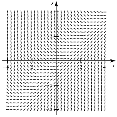
Direction fields The direction field for the equation y′(t)=t−y, for |t|≤4 and |y|≤4, is shown in the figure.
b. Use the direction field to sketch the solution curve that passes through the point (0,−1/2).