Back
BackProblem 2.1.1a
Average Rates of Change
In Exercises 1–6, find the average rate of change of the function over the given interval or intervals.
f(x)=x³+1
a. [2, 3]
Problem 2.1.3a
Average Rates of Change
In Exercises 1–6, find the average rate of change of the function over the given interval or intervals.
h(t)=cot t
a. [π/4,3π/4]
Problem 2.4.20a
Finding One-Sided Limits Algebraically
Find the limits in Exercises 11–20.
a. limx→0+ (1 − cos x) / |cos x − 1|
Problem 2.4.4a
Finding Limits Graphically
Let f(x) = {3 - x , x < 2
2, x = 2
x/2, x > 2
<IMAGE>
a. Find limx→2+ f(x), limx→2− f(x), and f(2).
Problem 2.7a
Limits and Continuity
On what intervals are the following functions continuous?
a. ƒ(x) = x¹/³
Problem 2.1.2a
Average Rates of Change
In Exercises 1–6, find the average rate of change of the function over the given interval or intervals.
g(x)=x²−2x
a. [1, 3]
Problem 2.6.61a
Find the limits in Exercises 59–62. Write ∞ or −∞ where appropriate.
lim ( 1 / x²/³ + 2 / (x − 1)²/³ ) as
a. x → 0⁺
Problem 2.2.68a
Estimating Limits
[Technology Exercise] You will find a graphing calculator useful for Exercises 67–74.
Let g(x) = (x² − 2) / (x − √2)
a. Make a table of the values of g at the points x=1.4,1.41,1.414, and so on through successive decimal approximations of √2. Estimate limx→√2 g(x).
Problem 2.5.6a
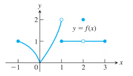
Exercises 5–10 refer to the function
f(x) = { x² − 1, −1 ≤ x < 0
2x, 0 < x < 1
1, x = 1
−2x + 4, 1 < x < 2
0, 2 < x < 3
graphed in the accompanying figure.
<IMAGE>
a. Does f (1) exist?
Problem 2.8a
Limits and Continuity
On what intervals are the following functions continuous?
a. ƒ(x) = tan x
Problem 2.29a
[Technology Exercise] Roots
Let ƒ(𝓍) = 𝓍³ ―𝓍― 1.
a. Use the Intermediate Value Theorem to show that ƒ has a zero between ―1 and 2 .
Problem 2.8b
Limits and Continuity
On what intervals are the following functions continuous?
b. g(x) = csc x
Problem 2.2.78b
Theory and Examples
If limx→−2 f(x) / x² = 1, find
b. limx→−2 f(x) / x
Problem 2.2.67b
Estimating Limits
[Technology Exercise] You will find a graphing calculator useful for Exercises 67–74.
Let f(x) = (x² - 9) / (x + 3)
b. Support your conclusions in part (a) by graphing f near c = -3 and using Zoom and Trace to estimate y-values on the graph as x → −3.
Problem 2.2.70b
Estimating Limits
[Technology Exercise] You will find a graphing calculator useful for Exercises 67–74.
Let h(x)=(x² − 2x − 3)/(x² − 4x + 3)
b. Support your conclusions in part (a) by graphing h near c = 3 and using Zoom and Trace to estimate y-values on the graph as x→3.
Problem 2.5.5b
Exercises 5–10 refer to the function
f(x) = { x² − 1, −1 ≤ x < 0
2x, 0 < x < 1
1, x = 1
−2x + 4, 1 < x < 2
0, 2 < x < 3
graphed in the accompanying figure.
<IMAGE>
b. Does lim x → −1⁺ f (x) exist?
Problem 2.6.45b
Infinite Limits
Find the limits in Exercises 37–48. Write ∞ or −∞ where appropriate.
b. lim x→0⁻ 2 / (3x¹/³)
Problem 2.2.69b
Estimating Limits
[Technology Exercise] You will find a graphing calculator useful for Exercises 67–74.
Let G(x)=(x + 6)/(x² + 4x − 12)
b. Support your conclusions in part (a) by graphing G and using Zoom and Trace to estimate y-values on the graph as x→−6.
Problem 2.2.55b
Suppose limx→b f(x) = 7 and lim x→b g(x) = −3. Find
b. limx→b f(x)⋅g(x)
Problem 2b
Finding Limits Graphically
Which of the following statements about the function y = f(x) graphed here are true, and which are false?
b. limx→2 f(x) does not exist
Problem 2.2.73b
Estimating Limits
[Technology Exercise] You will find a graphing calculator useful for Exercises 67–74.
Let g(θ) = (sinθ) / θ.
b. Support your conclusion in part (a) by graphing g near θ₀ = 0.
Problem 2.1.4b
Average Rates of Change
In Exercises 1–6, find the average rate of change of the function over the given interval or intervals.
g(t)=2+cos t
b. [0,π]
Problem 2.7b
Limits and Continuity
On what intervals are the following functions continuous?
b. g(x) = x³/⁴
Problem 2.2.72b
Estimating Limits
[Technology Exercise] You will find a graphing calculator useful for Exercises 67–74.
Let F(x)=(x² + 3x + 2)/(2−|x|)
b. Support your conclusion in part (a) by graphing F near c = -2 and using Zoom and Trace to estimate y-values on the graph as x→−2.
Problem 2.2.71b
Estimating Limits
[Technology Exercise] You will find a graphing calculator useful for Exercises 67–74.
Let f(x)=(x² − 1)/(|x| − 1).
b. Support your conclusion in part (a) by graphing f near c = -1 and using Zoom and Trace to estimate y-values on the graph as x→−1.
Problem 2.4.22b
Use the graph of the greatest integer function y = ⌊x⌋, Figure 1.10 in Section 1.1, to help you find the limits in Exercises 21 and 22.
<IMAGE>
b. limt→4−(t−⌊t⌋)
Problem 2.48c
Horizontal and Vertical Asymptotes
Use limits to determine the equations for all horizontal asymptotes.
_____
√x² + 4
c. g(x) = -----------
x
Problem 2.4.4c
Finding Limits Graphically
Let f(x) = {3 - x , x < 2
2, x = 2
x/2, x > 2
<IMAGE>
c. Find limx→−1− f(x) and limx→−1+ f(x).
Problem 2.47c
Horizontal and Vertical Asymptotes
Use limits to determine the equations for all vertical asymptotes.
x² + x ― 6
c. y = ------------------
x² + 2x ― 8
Problem 2.2.54c
Suppose limx→4 f(x) = 0 and lim x→4 g(x) = −3. Find
c. limx→4 (g(x))²