2–74. Integration techniques Use the methods introduced in Sections 8.1 through 8.5 to evaluate the following integrals.

54. ∫ dx/√(9x² - 25), x > 5/3

82-88. Improper integrals Evaluate the following integrals or show that the integral diverges.

86. ∫ (from -∞ to ∞) x³/(1 + x⁸) dx

89–91. Comparison Test Determine whether the following integrals converge or diverge.

89. ∫ (from 1 to ∞) dx/(x⁵ + x⁴ + x³ + 1)

2–74. Integration techniques Use the methods introduced in Sections 8.1 through 8.5 to evaluate the following integrals.

60. ∫ x² coshx dx

2–74. Integration techniques Use the methods introduced in Sections 8.1 through 8.5 to evaluate the following integrals.

9. ∫ (from 0 to π/4) cos⁵ 2x sin² 2x dx

82-88. Improper integrals Evaluate the following integrals or show that the integral diverges.

84. ∫ (from 0 to π) sec²x dx*(Note: Potential improperness at x = π/2)*

106. Arc length Find the length of the curve y = (x / 2) * sqrt(3 - x^2) + (3 / 2) * sin^(-1)(x / sqrt(3)) from x = 0 to x = 1.

118. Two worthy integrals

b. Let f be any positive continuous function on the interval [0, π/2]. Evaluate

∫ from 0 to π/2 of [f(cos x) / (f(cos x) + f(sin x))] dx.

(Hint: Use the identity cos(π/2 − x) = sin x.)

(Source: Mathematics Magazine 81, 2, Apr 2008)

2–74. Integration techniques Use the methods introduced in Sections 8.1 through 8.5 to evaluate the following integrals.

74. ∫ dx/√(√(1 + √x))

120. Equal volumes

a. Let R be the region bounded by the graph of f(x) = x^(-p) and the x-axis, for x ≥ 1. Let V₁ and V₂ be the volumes of the solids generated when R is revolved about the x-axis and the y-axis, respectively, if they exist. For what values of p (if any) is V₁ = V₂?

b. Repeat part (a) on the interval [0, 1].

119. {Use of Tech} Comparing volumes Let R be the region bounded by y = ln(x), the x-axis, and the line x = a, where a > 1.

b. Find the volume V₂(a) of the solid generated when R is revolved about the y-axis (as a function of a).

2–74. Integration techniques Use the methods introduced in Sections 8.1 through 8.5 to evaluate the following integrals.

48. ∫ sin(3x) cos⁶(3x) dx

2–74. Integration techniques Use the methods introduced in Sections 8.1 through 8.5 to evaluate the following integrals.

32. ∫ csc²(6x) cot(6x) dx

2–74. Integration techniques Use the methods introduced in Sections 8.1 through 8.5 to evaluate the following integrals.

6. ∫ (2 − sin 2θ)/cos² 2θ dθ

2–74. Integration techniques Use the methods introduced in Sections 8.1 through 8.5 to evaluate the following integrals.

29. ∫ cos⁴ x/sin⁶ x dx

2–74. Integration techniques Use the methods introduced in Sections 8.1 through 8.5 to evaluate the following integrals.

51. ∫ (from 0 to π/4) sin⁵(4θ) dθ

2–74. Integration techniques Use the methods introduced in Sections 8.1 through 8.5 to evaluate the following integrals.

22. ∫ tan³ 5θ dθ

Arc length of a parabola Let L(c) be the length of the parabola f(x) = x² from x = 0 to x = c, where c ≥ 0 is a constant.

a. Find an expression for L.

60. Two Methods

a. Evaluate ∫(x · ln(x²)) dx using the substitution u = x² and evaluating ∫(ln(u)) du.

41-44. {Use of Tech} Nonuniform grids

Use the indicated methods to solve the following problems with nonuniform grids.

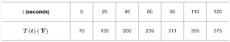
41. A curling iron is plugged into an outlet at time t = 0. Its temperature T in degrees Fahrenheit, assumed to be a continuous function that is strictly increasing and concave down on 0 ≤ t ≤ 120, is given at various times (in seconds) in the table.

a. Approximate (1/120)∫(0 to 120)T(t)dt in three ways using a left Riemann sum, using a right Riemann sum and using the Trapezoid Rule

Interpret the value of (1/120)∫(0 to 120)T(t)dt in the context of this problem.

66–71. {Use of Tech} Estimating error Refer to Theorem 8.1 in the following exercises.

70. Let f(x) = e^(-x²).

a. Find a Simpson's Rule approximation to the integral from 0 to 3 of e^(-x²) dx using n = 30 subintervals.

66–71. {Use of Tech} Estimating error Refer to Theorem 8.1 in the following exercises.

69. Let f(x) = sin(eˣ).

a. Find a Trapezoid Rule approximation to ∫[0 to 1] sin(eˣ) dx using n = 40 subintervals.

57. Explain why or why not Determine whether the following statements are true and give an explanation or counterexample.

a. If x = 4 tanθ, then cscθ = 4/x.

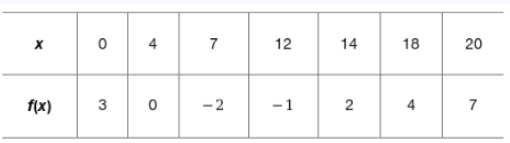
42. Approximating integrals The function f is twice differentiable on (-∞, ∞). Values of f at various points on [0, 20] are given in the table.

a. Approximate ∫(0 to 120) f(x) dx in three way using a left Riemann sum, a right Riemann sum and the Trapezoid Rule

81. Possible and impossible integrals

Let Iₙ = ∫ xⁿ e⁻ˣ² dx, where n is a nonnegative integer.

a. I₀ = ∫ e⁻ˣ² dx cannot be expressed in terms of elementary functions. Evaluate I₁.

Explain why or why not Determine whether the following statements are true and give an explanation or counterexample.

a. Suppose ∫_a^b f(x) dx is approximated with Simpson’s Rule using n = 18 subintervals, where |f^(4)(x)| ≤ 1 on [a, b]. The absolute error E_S in approximating the integral satisfies E_S ≤ (Δx)^5 / 10.

66–71. {Use of Tech} Estimating error Refer to Theorem 8.1 in the following exercises.

68. Let f(x) = e^(x²).

a. Find a Trapezoid Rule approximation to ∫[0 to 1] e^(x²) dx using n = 50 subintervals.

66–71. {Use of Tech} Estimating error Refer to Theorem 8.1 in the following exercises.

67. Let f(x) = √(x³ + 1).

a. Find a Midpoint Rule approximation to ∫[1 to 6] √(x³ + 1) dx using n = 50 subintervals.

Gamma function The gamma function is defined by Γ(p) = ∫ from 0 to ∞ of x^(p-1) e^(-x) dx, for p not equal to zero or a negative integer.

a. Use the reduction formula ∫ from 0 to ∞ of x^p e^(-x) dx = p ∫ from 0 to ∞ of x^(p-1) e^(-x) dx for p = 1, 2, 3, ...

to show that Γ(p + 1) = p! (p factorial).

91. [Use of Tech] Regions bounded by exponentials Let a > 0 and let R be the region bounded by the graph of y = e^(-a·x) and the x-axis

on the interval [b, ∞).

a. Find A(a,b), the area of R as a function of a and b.