15–16. {Use of Tech} Solving logistic equations Write a logistic equation with the following parameter values. Then solve the initial value problem and graph the solution. Let r be the natural growth rate, K the carrying capacity, and P₀ the initial population.

r=0.2, K=300, P₀=50

17–18. {Use of Tech} Designing logistic functions Use the method of Example 1 to find a logistic function that describes the following populations. Graph the population function.

The population increases from 50 to 60 in the first month and eventually levels off at 150.

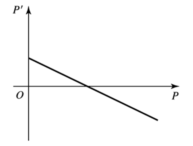
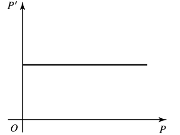
9–14. Growth rate functions Make a sketch of the population function P (as a function of time) that results from the following growth rate functions. Assume the population at time t = 0 begins at some positive value.

7–16. Verifying general solutions Verify that the given function is a solution of the differential equation that follows it. Assume C, C1, C2 and C3 are arbitrary constants.

u(t) = C₁t⁵ + C₂t⁻⁴ - t³; t²u''(t) - 20u(t) = 14t³

12–16. Sketching direction fields Use the window [-2, 2] x [-2, 2] to sketch a direction field for the following equations. Then sketch the solution curve that corresponds to the given initial condition. A detailed direction field is not needed.

y(x) = sin y, y(−2) = 1/2

17–20. Verifying solutions of initial value problems Verify that the given function y is a solution of the initial value problem that follows it.

y(t) = 8t⁶ - 3; ty'(t) - 6y(t) = 18, y(1) = 5

Does the function y(t) = 2t satisfy the differential equation y'''(t) + y'(t) = 2?

9–14. Growth rate functions Make a sketch of the population function P (as a function of time) that results from the following growth rate functions. Assume the population at time t = 0 begins at some positive value.

27–30. Newton’s Law of Cooling Solve the differential equation for Newton’s Law of Cooling to find the temperature function in the following cases. Then answer any additional questions.

A pot of boiling soup (100°C) is put in a cellar with a temperature of 10°C. After 30 minutes, the soup has cooled to 80°C. When will the temperature of the soup reach 30°C 

​​​​​​​​What is a separable first-order differential equation?

Soluti​​on of the logistic equation Use separation of variables to show that the solution of the initial value problem

P'(t) = rP (1-P/K), P(0) = P₀

is P(t) = K/((K/P₀ − 1)e⁻ʳᵗ + 1)

5–16. Solving separable equations Find the general solution of the following equations. Express the solution explicitly as a function of the independent variable.

u'(x) = e²ˣ⁻ᵘ

33–38. {Use of Tech} Solutions in implicit form Solve the following initial value problems and leave the solution in implicit form. Use graphing software to plot the solution. If the implicit solution describes more than one function, be sure to indicate which function corresponds to the solution of the initial value problem.

y'(t) = 2t²/(y² − 1), y(0) = 0

Stability of Euler's method Consider the initial value problem y′(t) = −ay, y(0) = 1 where a > 0; it has the exact solution y(t) = e⁻ᵃᵗ, which is a decreasing function.

a. Show that Euler's method applied to this problem with time step h can be written u₀ = 1, uₖ₊₁ = (1 − ah)uₖ for k = 0, 1, 2, ...

b. Show by substitution that uₖ = (1 − ah)ᵏ is a solution of the equations in part (a), for k = 0, 1, 2, ...

Case 2 of the general solution Solve the equation y′(t) = ky + b in the case that ky + b < 0 and verify that the general solution is y(t) = Ceᵏᵗ − b/k.

Explain how to solve a separable differential equation of the form

g(t)y'(y) = h(t)

45–46. Harvesting problems Consider the harvesting problem in Example 6.

If r = 0.05 and H = 500, for what values of p₀ is the amount of the resource decreasing? For what value of p₀ is the amount of the resource constant? If p₀ = 9000, when does the resource vanish?

21–24. Logistic equations Consider the following logistic equations. In each case, sketch the direction field, draw the solution curve for each initial condition, and find the equilibrium solutions. A detailed direction field is not needed. Assume t ≥ 0 and tP ≥ 0.

P′(t) = 0.05P − 0.001P²; P(0) = 10, P(0) = 40, P(0) = 80

5–16. Solving separable equations Find the general solution of the following equations. Express the solution explicitly as a function of the independent variable.

(t² + 1)³yy'(t) = t(y² + 4)

17–32. Solving initial value problems Determine whether the following equations are separable. If so, solve the initial value problem.

y'(t) = yeᵗ, y(0) = −1

The general solution of a first-order linear differential equation is y(t) = Ce⁻¹⁰ᵗ − 13. What solution satisfies the initial condition y(0) = 4?

Explain why the graph of the solution to the initial value problem y'(t) = t²/(1 - t), y(-1) = ln 2 cannot cross the line t = 1.

11–16. Initial value problems Solve the following initial value problems.

y'(t) − 3y = 12, y(1) = 4

20–22. {Use of Tech} Solving the Gompertz equation Solve the Gompertz equation in Exercise 19 with the given values of r, K, and M₀. Then graph the solution to be sure that M(0) and lim(t→∞) M(t) are correct.

r = 0.05, K = 1200, M₀ = 90

33–42. Solving initial value problems Solve the following initial value problems.​

y'(x) = 4 sec² 2x, y(0) = 8

12–16. Sketching direction fields Use the window [-2, 2] x [-2, 2] to sketch a direction field for the following equations. Then sketch the solution curve that corresponds to the given initial condition. A detailed direction field is not needed.

y'(t) = 4−y, y(0) = −1

27–30. Newton’s Law of Cooling Solve the differential equation for Newton’s Law of Cooling to find the temperature function in the following cases. Then answer any additional questions.

An iron rod is removed from a blacksmith’s forge at a temperature of 900°C . Assume k=0.02 and the rod cools in a room with a temperature of 30°C When does the temperature of the rod reach 100°C? 

What is the equilibrium solution of the equation y'(t) = 3y − 9? Is it stable or unstable?

Orthogonal trajectories Use the method in Exercise 44 to find the orthogonal trajectories for the family of circles x² + y² = a²

33–42. Solving initial value problems Solve the following initial value problems.​

y'(t) = 1 + eᵗ, y(0) = 4