7–16. Verifying general solutions Verify that the given function is a solution of the differential equation that follows it. Assume C, C1, C2 and C3 are arbitrary constants.

y(t) = C₁ sin4t + C₂ cos4t; y''(t) + 16y(t) = 0

33–42. Solving initial value problems Solve the following initial value problems.​

y'(t) = 1 + eᵗ, y(0) = 4

Logistic growth in India The population of India was 435 million in 1960 (t=0) and 487 million in 1965 (t=5). The projected population for 2050 is 1.57 billion.

b. Use the solution of the logistic equation and the 2050 projected population to determine the carrying capacity.

11–18. Solving initial value problems Use the method of your choice to find the solution of the following initial value problems.

y′(t) = -3y + 9, y(0) = 4

A first-order equation Consider the equation t² y′(t) + 2ty(t) = e⁻ᵗ

c. Find the solution that satisfies the condition y(1) = 0

A predator-prey model Consider the predator-prey model

x′(t) = −4x + 2xy, y′(t) = 5y − xy

c. Find the equilibrium points for the system.

2–10. General solutions Use the method of your choice to find the general solution of the following differential equations.

y′(t) = √(y/t)

A second-order equation Consider the equation

t² y′′(t) + 2ty′(t) − 12y(t) = 0

b. Assuming the general solution of the equation is

y(t) = C₁ tᵖ¹ + C₂ tᵖ²,

find the solution that satisfies the conditions

y(1) = 0, y′(1) = 7

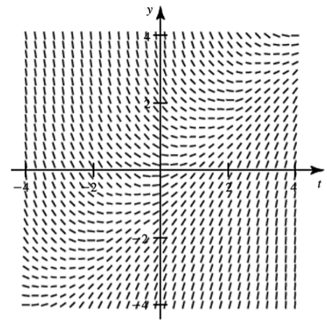
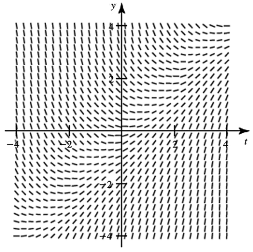
Direction fields Consider the direction field for the equation y′=y(2−y) shown in the figure and initial conditions of the form y(0)=A.

a. Sketch a solution on the direction field with the initial condition y(0)=1.

Logistic growth in India The population of India was 435 million in 1960 (t=0) and 487 million in 1965 (t=5). The projected population for 2050 is 1.57 billion.

e. Discuss some possible shortcomings of this model. Why might the carrying capacity be either greater than or less than the value predicted by the model?

Direction fields Consider the direction field for the equation y′=y(2−y) shown in the figure and initial conditions of the form y(0)=A.

d. For what values of A are the corresponding solutions decreasing, for t≥0

Logistic growth parameters A cell culture has a population of 20 when a nutrient solution is added at t=0. After 20 hours, the cell population is 80 and the carrying capacity of the culture is estimated to be 1600 cells.

c. After how many hours does the population reach half of the carrying capacity

A first-order equation Consider the equation t² y′(t) + 2ty(t) = e⁻ᵗ

a. Show that the left side of the equation can be written as the derivative of a single term.

2–10. General solutions Use the method of your choice to find the general solution of the following differential equations.

y′(t) = (2t+1)(y²+1)

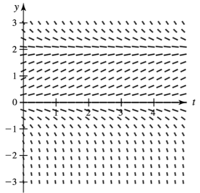
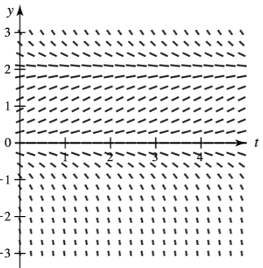
Direction fields The direction field for the equation y′(t)=t−y, for |t|≤4 and |y|≤4, is shown in the figure.

b. Use the direction field to sketch the solution curve that passes through the point (0,−1/2).

11–18. Solving initial value problems Use the method of your choice to find the solution of the following initial value problems.

y′(x) = 4x csc y, y(0) = π/2

Logistic growth The population of a rabbit community is governed by the initial value problem

P′(t) = 0.2 P (1 − P/1200), P(0) = 50

d. What is the population when the growth rate is a maximum?

Euler’s method Consider the initial value problem y′(t)=1/2y,y(0)=1. 

b. Use Euler’s method with Δt=0.05 to compute approximations to y(0.1) and y(0.2). 

2–10. General solutions Use the method of your choice to find the general solution of the following differential equations.

y′(t) + 2y = 6

Direction fields The direction field for the equation y′(t)=t−y, for |t|≤4 and |y|≤4, is shown in the figure.

d. Complete the following sentence. The solution of the differential equation with the initial condition y(0)=A, where A is a real number, approaches the line _____ as t→∞.

Euler’s metho d Consider the initial value problem y′(t)=1/2y,y(0)=1. 

a. Use Euler’s method with Δt=0.1 to compute approximations to y(0.1) and y(0.2). 

Newton’s Law of Cooling A cup of coffee is removed from a microwave oven with a temperature of 80°C and allowed to cool in a room with a temperature of 25°C. Five minutes later, the temperature of the coffee is 60°C.

c. When does the temperature of the coffee reach 50°C?

11–18. Solving initial value problems Use the method of your choice to find the solution of the following initial value problems.

y′(x) = x/y, y(2) = 4

22–25. Equilibrium solutions Find the equilibrium solutions of the following equations and determine whether each solution is stable or unstable.

y′(t) = y(3+y)(y-5)

Logistic growth The population of a rabbit community is governed by the initial value problem

P′(t) = 0.2 P (1 − P/1200), P(0) = 50

a. Find the equilibrium solutions.

Stirred tank reaction A 100-L tank is filled with pure water when an inflow pipe is opened and a sugar solution with a concentration of 20 gm/L flows into the tank at a rate of 0.5 L/min. The solution is thoroughly mixed and flows out of the tank at a rate of 0.5 L/min.

c. At what time does the mass of sugar reach 95% of its steady-state level?

Explain why or why not Determine whether the following statements are true and give an explanation or counterexample.

d. The direction field for the differential equation y′(t)=t+y(t) is plotted in the ty-plane.

Explain why or why not Determine whether the following statements are true and give an explanation or counterexample.

a. The differential equation y′+2y=t is first-order, linear, and separable.

43–44. Motion in a gravitational field: An object is fired vertically upward with initial velocity v(0)=v₀ from initial position s(0)=s₀.

a. For the following values of v₀ and s₀, find the position and velocity functions for all times at which the object is above the ground (s = 0).

v₀ = 49 m/s, s₀ = 60 m

Consider the differential equation y'(t)+9y(t)=10.

a. How many arbitrary constants appear in the general solution of the differential equation?